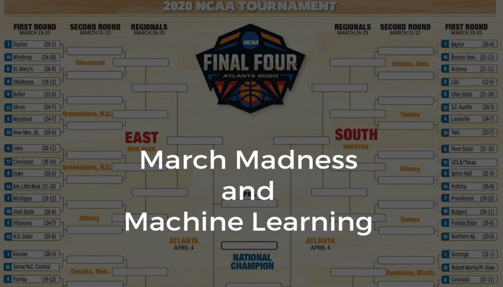
Both the March Madness basketball tournament and the Kaggle competition – which predicts the winner of the tournament based on machine learning techniques – were canceled this year. That is unfortunate as not only did the public miss out on some of the year’s best basketball, but programmers also missed out on a great way to advance our skills, sharpen our data-wrangling capabilities, and expand our machine learning (ML) horizons.
But while the seventh annual Kaggle-hosted Google Cloud and NCAA March Madness competition has been cancelled, we can still create a model against past tournament data and even see how it can be applied to this year’s tournament. Kaggle supplies datasets composed of the NCAA basketball’s historical data, already cleaned and ready for competitors to sift through in order to create a suitable algorithm for predicting the winners of each round. The dataset is relatively large, and much of the information may not be useful, but it is up to the participants to determine this.
In this tutorial, I will guide you through the steps to create a predictive algorithm using common ML techniques, all the way from the initial installation of Python and all the libraries we’ll need to:
- Importing and exploring the dataset
- Feature engineering
- Creating a test and training set
- Assessing different ML models
And finally, even though the competition is cancelled, I’ll show how to prepare a set of predictions against a mock 2020 March Madness tournament so you’ll be all set for next year’s competition.
March Madness 2020 runtime environment
To follow along with the code in this tutorial, you’ll need to have a recent version of Python installed. When starting a new project, it’s always best to begin with a clean implementation in a virtual environment. You have two choices:Download the pre-built March Madness 2020 runtime environment (including Python 3.6) for Windows 10, Linux or macOS and install it using the State Tool into a virtual environment, or
Build your own custom Python runtime by making a free account and creating a project on the ActiveState Platform:
Choose a version of Python
Select the Platform you work on
Add the required ML packages, including numpy, scipy, scikit-learn and xgboost.
Press Commit, and then install the build with the State Tool after it completes.
All set? Let’s dive into the details.
Competition Details
The competition normally consists of two stages:
- Historical NCAA data from the regular season and tournament play going back to 1985 is used to predict probabilities for every possible matchup in the past 5 NCAA tournaments (seasons 2015-2019). During this stage, submitted models are evaluated on how well they predict the results of these tournaments.
- After the release of the official tournament brackets on March 15th, competitors typically use the model developed in the first stage to predict the win probabilities of every possible matchup of the 68 participating teams.
The data provided is broken up into six parts:
- Basic Data: This section is composed of six files containing basic information on all teams, such as how they are ranked in each season, as well as how they have performed during the regular season and in the tournament. It also includes a sample submission file that will serves as a template for our own predictions.
- Team Box Scores: The team box scores consist of game statistics at a team level for the regular season and tournament games going back to the 2003 season. These statistics include metrics such as free throws attempted, defensive rebounds, turnovers, etc.
- Geography: All geographical information on where games are played, from the regular season and tournament. The data goes back to the 2010 season.
- Public Rankings: Public rankings of each team are released on a weekly basis by professional analysts and entities. These are compiled into a single file going back to the 2003 season.
- Play-by-Play: This consists of six files, each containing play-by-play statistics of the regular season and tournament games from the 2015 to 2019 seasons. These track in-game events such as assists, blocks, fouls, and others, at exactly the time they occur and by which player.
- Supplements: These files contain any supplemental information such as coaches, conferences, bracket structures, and the results of other postseason tournaments.
In addition to this data, incorporating external data is not only allowed, it is encouraged. The provided data is subject to updates throughout the first stage of the competition, as some of the information, such as the public rankings, change as the start of the tournament approaches. Everything can be downloaded here. Additionally, a more in-depth look at the data can be found on the same page.
Approaching the Problem
Before deciding on how to approach building a model, it can be useful to obtain a qualitative understanding of the data. In many cases, the physical significance of each data feature is undisclosed, so we are forced to discover any correlations through an exploratory analysis. Typically, this is the first task to be done once the data has been imported.
Fortunately, basketball is a relatively popular game, and as a result, an exhaustive amount of qualitative and quantitative analysis are publicly available. Even with a basic understanding of the game, identifying the key metrics that determine success is simple. If the goal of the model is to predict the win probabilities of each possible matchup in the tournament, the most important question to answer is: Which statistical metrics determine whether a team wins or not?
If you are unfamiliar with college basketball, I recommend reading the tournament wikipedia page here. The standard in-game metrics of basketball are a good place to start building our model. The number of points scored during a game by each team determines the winner, so the average number of points scored per game by each team is probably an important factor. There are several other offensive and defensive metrics that are correlated with increasing the chance of a team winning, including:
- Offensive rebounds and assists. Offensive rebounds give the team on offense another possession and chance to score, and assists promote scoring opportunities.
- Forcing a turnover, getting a steal, or making a defensive rebound all prevent the opposing team from scoring and result in a change of possession.
- The number of missed shots an offense makes also may be a good metric to evaluate the opposing defense.
In addition to the in-game metrics, we can incorporate third-party rankings into the model. There are many third-parties that spend a lot of time and money to perform their own analysis and rank the teams as the season progresses. The public rankings that are available on Kaggle are compiled by Kenneth Massey and provided on his College Basketball Ranking Composite page. There are several different ranking systems, each with their own method. Our model should take advantage of these rankings.
The strategy here is to construct a dataset where each row represents a single game, with each column representing one or several of the previously mentioned metrics for each team. The result of each game can be represented by a binary 0 or 1, where 0 represents a Team 2 victory and 1 a Team 1 victory. For the first stage of the competition, we can build test and training sets for the 2015 to 2019 seasons to identify which features we should include in the model. The predicted value will be a number from 0 to 1 that represents the probability of Team 1 beating Team 2.
For the second stage of the competition, we’ll use the mock tournament bracket published by the New York post in order to predict the win probabilities of the 2020 tournament. The best data to use to predict this is data from the 2020 regular season; perhaps even just the last few weeks of the regular season. So, our test set will be all possible matchups of the 2020 tournament teams, and our training set will be games that occur in the 2020 regular season. We could easily include games from previous seasons, but they may hinder the model more than help, as the players on each team change from year to year.
Feature Engineering
As is true of most problems within data science, there are many different approaches, each of which will have varying degrees of success. This post presents the entire model construction as a single process, when in reality each stage is iterative. Generally, creating the pipeline of data importation, feature engineering, model training and testing is the first step. This is followed by cycling back through each stage and making modifications (adding new data, creating new features, tuning model parameters, etc.) to improve the model.
In order to be prepared for the tight submission window of Stage 2, any data manipulation that we performed on the data from the 2015 to 2019 seasons would have needed to be performed on the 2020 season rather quickly once it would have been released on March 16th. So, we wrote a generalized function for each feature engineering step that contained all the manipulations implemented for each year. This would have allowed us to process the 2020 data immediately, without writing any additional lines of code.
To get started, let’s import the relevant data from the 2015 to 2019 regular season and tournament. This is data from the Basic Data, Team Box Scores, and Public Rankings sections:
import pandas as pd
import numpy as np
tcr_df = pd.read_csv('google-cloud-ncaa-march-madness-2020-division-1-mens-tournament/Basics/MNCAATourneyCompactResults.csv')
ts_df = pd.read_csv('google-cloud-ncaa-march-madness-2020-division-1-mens-tournament/Basics/MNCAATourneySeeds.csv')
rscr_df = pd.read_csv('google-cloud-ncaa-march-madness-2020-division-1-mens-tournament/Basics/MRegularSeasonCompactResults.csv')
ss_df = pd.read_csv('google-cloud-ncaa-march-madness-2020-division-1-mens-tournament/Basics/MSampleSubmissionStage1_2020.csv')
massey_df = pd.read_csv('google-cloud-ncaa-march-madness-2020-division-1-mens-tournament/PublicRankings/MMasseyOrdinals.csv')
tbs_df = pd.read_csv('google-cloud-ncaa-march-madness-2020-division-1-mens-tournament/TeamBoxScores/MNCAATourneyDetailedResults.csv')
rsbs_df = pd.read_csv('google-cloud-ncaa-march-madness-2020-division-1-mens-tournament/TeamBoxScores/MRegularSeasonDetailedResults.csv')
The first features we extract are average points-per-game (PPG) for each season, the season win percentage, and total games played with a user-defined function get_ppg(). The dataframe from the MRegularSeasonCompactResults.csv serves as the input. This dataframe looks like the following:
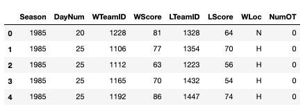
Each row is a single game with the winning team statistics (the columns starting with W) and the losing team statistics (the columns starting with L). The function below contains the different manipulations we performed to extract the relevant data. First we normalized the number of points scored in a game to account for games that go into overtime (otherwise, the points-per-game statistic is overestimated for the teams that play more overtimes). Then we averaged the points-per-game across every game in each season. We also calculated the number of games in each season and win percentage for the season.
def get_ppg(rscr_df):
    #Gametime normalization
    rscr_df['GameDuration'] = rscr_df['NumOT']
    for i in range(len(rscr_df.NumOT.value_counts())):
        rscr_df.loc[rscr_df['NumOT'] == rscr_df.NumOT.value_counts().index[i], 'GameDuration'] = 40 + i*5
    rscr_df['Wppg'] = (rscr_df['WScore'] / rscr_df['GameDuration']) * 40
    rscr_df['Lppg'] = (rscr_df['LScore'] / rscr_df['GameDuration']) * 40
    #Drop unnecesary columns
    rscr_df = rscr_df.drop(['DayNum', 'WLoc', 'NumOT', 'WScore','LScore','GameDuration'], axis = 1)
    #Calculate average points per game and number of games for winning and losing team
    Wppg_df = rscr_df[["Season","WTeamID",'Wppg']].groupby(["Season","WTeamID"]).agg(['mean', 'count'])
    Lppg_df = rscr_df[["Season","LTeamID",'Lppg']].groupby(["Season","LTeamID"]).agg(['mean', 'count'])
    Wppg_df.columns = Wppg_df.columns.droplevel(0)
    Wppg_df = Wppg_df.reset_index().rename(columns = {'mean':'Wppg', 'count':'WGames'})
    Lppg_df.columns = Lppg_df.columns.droplevel(0)
    Lppg_df = Lppg_df.reset_index().rename(columns = {'mean':'Lppg', 'count':'LGames'})
    #Merge PPG for wins and losses and fill NaNs with 0s for undefeated and no-win teams
    ppg_df = pd.merge(Wppg_df, Lppg_df, left_on=['Season', 'WTeamID'], right_on=['Season', 'LTeamID'], how='outer')
    ppg_df = ppg_df.fillna({'WTeamID': ppg_df.LTeamID, 'Wppg': 0, 'WGames': 0, 'LTeamID': ppg_df.WTeamID , 'Lppg': 0, 'LGames': 0})
    #Calculate PPG and win percentage for season
    ppg_df['PPG'] = (ppg_df['Wppg']*ppg_df['WGames'] + ppg_df['Lppg']*ppg_df['LGames'])/(ppg_df['WGames'] + ppg_df['LGames'])
    ppg_df['WPerc'] = (ppg_df['WGames'])/(ppg_df['WGames'] + ppg_df['LGames'])
    ppg_df['TeamID'] = ppg_df['WTeamID'].astype('int32')
    ppg_df['GamesPlayed'] = (ppg_df['WGames'] + ppg_df['LGames'])
    ppg_df = ppg_df.drop(['WTeamID', 'Wppg' ,'WGames','LTeamID', 'Lppg','LGames'],axis = 1)
    return ppg_df
The output dataframe looks like the following:
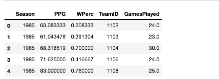
So, this gave us a nice clean dataframe with the win percentage, points-per-game, and number of games played for each team and season. Next, we looked to extract more in- depth game metrics from the MRegularSeasonDetailedResults.csv file. This file contains metrics like assists, steals, rebounds, and others for each team. This data looks like:

A few of the columns were identical to those we pulled from the MRegularSeasonCompactResults.csv file, so we didn’t need those. Instead, we focused on creating an offensive and defensive efficiency metric for each team:
- Offensive Efficiency – metrics commonly used among professional basketball analysts to characterize how well a team converts possessions to points.
- Defensive Efficiency – how well a team prevents the opposing team’s possessions from becoming points.
Calculating efficiencies usually involves boiling down multiple game statistics to produce a single statistic. The exact method of doing so varies from analyst to analyst, and even league to league. A few common ways are described here (usually a linear combination of the base statistics). Using a single statistic is also advantageous from an ML perspective, as the fewer features we have in our model, the less likely we are to encounter poor model performance due to the curse of dimensionality.
In the function below, I created an offensive metric based on points made, assists, and offensive rebounds, as well as a defensive metric based on opposing team points missed, steals, defensive rebounds, turnovers forced, blocks, and personal fouls. I averaged the metrics across the entire regular season, and also the last 30 days of the season.
def get_efficiency(rsbs_df):
    #Gametime normalization
    rsbs_df['GameDuration'] = rsbs_df['NumOT']
    for i in range(len(rsbs_df.NumOT.value_counts())):
        rsbs_df.loc[rsbs_df['NumOT'] == rsbs_df.NumOT.value_counts().index[i], 'GameDuration'] = 40 + i*5
    rsbs_df['WFGM'] = (rsbs_df['WFGM'] / rsbs_df['GameDuration']) * 40
    rsbs_df['WFGA'] = (rsbs_df['WFGA'] / rsbs_df['GameDuration']) * 40
    rsbs_df['WFGM3'] = (rsbs_df['WFGM3'] / rsbs_df['GameDuration']) * 40
    rsbs_df['WFGA3'] = (rsbs_df['WFGA3'] / rsbs_df['GameDuration']) * 40
    rsbs_df['WFTM'] = (rsbs_df['WFTM'] / rsbs_df['GameDuration']) * 40
    rsbs_df['WFTA'] = (rsbs_df['WFTA'] / rsbs_df['GameDuration']) * 40
    rsbs_df['WOR'] = (rsbs_df['WOR'] / rsbs_df['GameDuration']) * 40
    rsbs_df['WDR'] = (rsbs_df['WDR'] / rsbs_df['GameDuration']) * 40
    rsbs_df['WAst'] = (rsbs_df['WAst'] / rsbs_df['GameDuration']) * 40
    rsbs_df['WTO'] = (rsbs_df['WTO'] / rsbs_df['GameDuration']) * 40
    rsbs_df['WStl'] = (rsbs_df['WStl'] / rsbs_df['GameDuration']) * 40
    rsbs_df['WBlk'] = (rsbs_df['WBlk'] / rsbs_df['GameDuration']) * 40
    rsbs_df['WPF'] = (rsbs_df['WPF'] / rsbs_df['GameDuration']) * 40
    rsbs_df['LFGM'] = (rsbs_df['LFGM'] / rsbs_df['GameDuration']) * 40
    rsbs_df['LFGA'] = (rsbs_df['LFGA'] / rsbs_df['GameDuration']) * 40
    rsbs_df['LFGM3'] = (rsbs_df['LFGM3'] / rsbs_df['GameDuration']) * 40
    rsbs_df['LFGA3'] = (rsbs_df['LFGA3'] / rsbs_df['GameDuration']) * 40
    rsbs_df['LFTM'] = (rsbs_df['LFTM'] / rsbs_df['GameDuration']) * 40
    rsbs_df['LFTA'] = (rsbs_df['LFTA'] / rsbs_df['GameDuration']) * 40
    rsbs_df['LOR'] = (rsbs_df['LOR'] / rsbs_df['GameDuration']) * 40
    rsbs_df['LDR'] = (rsbs_df['LDR'] / rsbs_df['GameDuration']) * 40
    rsbs_df['LAst'] = (rsbs_df['LAst'] / rsbs_df['GameDuration']) * 40
    rsbs_df['LTO'] = (rsbs_df['LTO'] / rsbs_df['GameDuration']) * 40
    rsbs_df['LStl'] = (rsbs_df['LStl'] / rsbs_df['GameDuration']) * 40
    rsbs_df['LBlk'] = (rsbs_df['LBlk'] / rsbs_df['GameDuration']) * 40
    rsbs_df['LPF'] = (rsbs_df['LPF'] / rsbs_df['GameDuration']) * 40
    #Calculate total points made and missed per game
    rsbs_df['wPointsMade'] = (2* (rsbs_df['WFGM'] - rsbs_df['WFGM3'])) + 3*rsbs_df['WFGM3'] + rsbs_df['WFTM']
    rsbs_df['wPointsMissed'] = (2* (rsbs_df['WFGA'] - rsbs_df['WFGA3'])) + 3*rsbs_df['WFGA3'] + rsbs_df['WFTA'] - rsbs_df['wPointsMade']
    rsbs_df['lPointsMade'] = (2* (rsbs_df['LFGM'] - rsbs_df['LFGM3'])) + 3*rsbs_df['LFGM3'] + rsbs_df['LFTM']
    rsbs_df['lPointsMissed'] = (2* (rsbs_df['LFGA'] - rsbs_df['LFGA3'])) + 3*rsbs_df['LFGA3'] + rsbs_df['LFTA'] - rsbs_df['lPointsMade']
    #Calculate offensive and defensive efficiency metrics for winning and losing team
    rsbs_df['WoEFF'] = rsbs_df['wPointsMade'] +  rsbs_df['WAst'] + rsbs_df['WOR']
    rsbs_df['WdEFF'] = rsbs_df['lPointsMissed'] + rsbs_df['WStl'] + rsbs_df['WBlk'] + rsbs_df['WDR'] + rsbs_df['LTO'] - rsbs_df['WPF']
    rsbs_df['LoEFF'] = rsbs_df['lPointsMade'] +  rsbs_df['LAst'] + rsbs_df['LOR']
    rsbs_df['LdEFF'] = rsbs_df['wPointsMissed'] + rsbs_df['LStl'] + rsbs_df['LBlk'] + rsbs_df['LDR'] + rsbs_df['WTO'] - rsbs_df['LPF']
    #Extract relevant columns and rename
    Weff_df = rsbs_df[['Season', 'DayNum', 'WTeamID','WoEFF', 'WdEFF']]
    Weff_df = Weff_df.rename(columns = {'WTeamID': 'TeamID','WoEFF': 'oEFF', 'WdEFF': 'dEFF'})
    Leff_df = rsbs_df[['Season', 'DayNum', 'LTeamID','LoEFF', 'LdEFF']]
    Leff_df = Leff_df.rename(columns = {'LTeamID': 'TeamID','LoEFF': 'oEFF', 'LdEFF': 'dEFF'})
    eff_df = pd.concat([Weff_df, Leff_df])
    #Take seasonal and 30 day averages of the efficiency metrics
    effseas_df = eff_df.groupby(by = ['Season', 'TeamID']).agg('mean').reset_index().drop(['DayNum'], axis = 1)
    eff30day_df = eff_df[eff_df.DayNum >= 100].groupby(by = ['Season', 'TeamID']).agg('mean').reset_index().drop(['DayNum'], axis = 1)
    eff30day_df = eff30day_df.rename(columns = {'oEFF': 'oEFF_30day', 'dEFF': 'dEFF_30day' })
    eff_df = pd.merge(effseas_df,eff30day_df, how = 'outer', on = ['Season', 'TeamID'])
    return eff_df
The dataframe output looks like this:
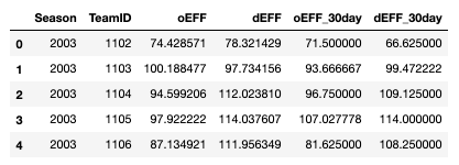
My hope is that the 30-day efficiency metrics more accurately capture how ‘hot’ a team is, going into the tournament.
From here, we moved on to the rankings data. After import, the MMasseyOrdinals.csv file looks like this:
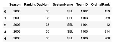
Because we’re interested in the ranking right before the tournament would have begun, we only extracted rankings with the RankingDayNum column equal to 133 (corresponding to the last day of the regular season). Different rankings are known to have a better reputation than others (some being more conservative, others giving preference to certain coaches or divisions), so I took the median and mean rank of each team across all rankings. I also singled out the Massey ranking, as it is known to be objective and accurate.
def get_rank(massey_df):
    rankings_df = massey_df[massey_df['RankingDayNum'] == 133]
    rankings_df = rankings_df.reset_index().drop(['index','RankingDayNum'], axis = 1)
    median_df = rankings_df.groupby(by = ['Season','TeamID'])[['OrdinalRank']].median().reset_index()
    median_df = median_df.rename(columns = {'OrdinalRank':'MedianRank'})
    mean_df = rankings_df.groupby(by = ['Season','TeamID'])[['OrdinalRank']].mean().reset_index()
    mean_df = mean_df.rename(columns = {'OrdinalRank':'MeanRank'})
    massey_df = rankings_df[rankings_df['SystemName'] == 'MAS']
    massey_df = massey_df.reset_index().drop(['index','SystemName'], axis = 1)
    massey_df = massey_df.rename(columns = {'OrdinalRank':'MasseyRank'})
    rankings_df = pd.merge(median_df, massey_df, left_on=['Season', 'TeamID'], right_on=['Season', 'TeamID'], how='left')
    rankings_df = pd.merge(rankings_df, mean_df, left_on=['Season', 'TeamID'], right_on=['Season', 'TeamID'], how='left')
    return rankings_df
The output dataframe looks like this:
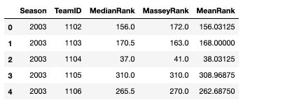
Thus far, we have defined three functions that produce three dataframes containing our basic metrics, efficiency metrics, and rankings. Now, we need to define a function that merges them all together.
Before doing that, we should construct a dataframe with the correct submission structure to merge our features onto. Thankfully, Kaggle provides a sample submission file that we can use as a template. The first few rows of the sample look like the following:
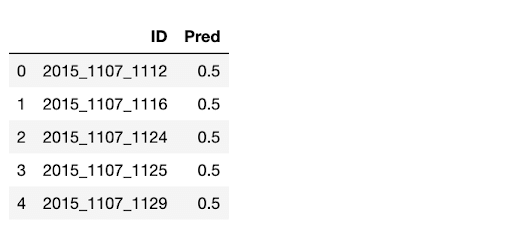
Where each row represents a matchup in the tournament for each season. The ID consists of the season, the lower Team ID, and the higher Team ID. The Pred column corresponds to the predicted probability of the lower Team ID beating the higher Team ID. Within the context of our model, we used the features we engineered to predict this column. Then, we compared the prediction to the actual result.
The functions below prepare the sample submission file so that we could merge these features onto it:
def prep_submission(ss_df,tcr_df):
    features_df = ss_df.copy()
    #extract season and team IDs
    features_df['Season'] = features_df['ID'].map(lambda x: int(x[:4]))
    features_df['WTeamID'] = features_df['ID'].map(lambda x: int(x[5:9]))
    features_df['LTeamID'] = features_df['ID'].map(lambda x: int(x[10:14]))
    features_df = features_df.rename(columns= {'WTeamID':'TeamID_1','LTeamID':'TeamID_2'})
    #Extract seasons starting from 2015 and create Result column corresponding to winner and loser
    Wtcr_df = tcr_df[tcr_df.Season >= 2015].loc[:,['Season', 'WTeamID', 'LTeamID']].reset_index().drop('index', axis = 1)
    Wtcr_df = Wtcr_df.rename(columns = {'WTeamID': 'TeamID_1', 'LTeamID': 'TeamID_2'})
    Wtcr_df['Result'] = 1
    Ltcr_df = tcr_df[tcr_df.Season >= 2015].loc[:,['Season', 'WTeamID', 'LTeamID']].reset_index().drop('index', axis = 1)
    Ltcr_df = Ltcr_df.rename(columns = {'WTeamID': 'TeamID_2', 'LTeamID': 'TeamID_1'})
    Ltcr_df['Result'] = 0
    tcr_df = pd.concat([Wtcr_df,Ltcr_df], sort=False).reset_index().drop('index', axis = 1)
    tcr_df['ID'] = tcr_df['Season'].apply(str) + '_' + tcr_df['TeamID_1'].apply(str) + '_' + tcr_df['TeamID_2'].apply(str)
    tcr_df = tcr_df.drop(['Season', 'TeamID_1', 'TeamID_2'],axis = 1)
    #merge results onto sample submission
    features_df = pd.merge(features_df,tcr_df, how = 'left', on = 'ID')
    features_df = features_df.drop(['Pred'],axis = 1)
    return features_df
Test & Training Sets
Besides generating a sample submission file, the above function also creates our test set, which corresponds to all possible tournament matchups for each of the past season’s tournaments. The output looks like this:
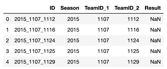
Note that many of the results are NaN. This is not surprising, as we are meant to predict ALL possible matchups, not just the games that were actually played. Unfortunately, this implies that we can only use the matchups that actually happened to evaluate how well our predictive model performs.
We can create our training set (regular season games) in much the same way:
def prep_regseason(rscr_df):
    #Extract seasons starting from 2015 and create Result column corresponding to winner and loser
    Wrscr_df = rscr_df[rscr_df.Season >= 2015].loc[:,['Season', 'WTeamID', 'LTeamID']].reset_index().drop('index', axis = 1)
    Wrscr_df = Wrscr_df.rename(columns = {'WTeamID': 'TeamID_1', 'LTeamID': 'TeamID_2'})
    Wrscr_df['Result'] = 1
    Lrscr_df = rscr_df[rscr_df.Season >= 2015].loc[:,['Season', 'WTeamID', 'LTeamID']].reset_index().drop('index', axis = 1)
    Lrscr_df = Lrscr_df.rename(columns = {'WTeamID': 'TeamID_2', 'LTeamID': 'TeamID_1'})
    Lrscr_df['Result'] = 0
    rscr_df = pd.concat([Wrscr_df,Lrscr_df], sort=False).reset_index().drop('index', axis = 1)
    rscr_df['ID'] = rscr_df['Season'].apply(str) + '_' + rscr_df['TeamID_1'].apply(str) + '_' + rscr_df['TeamID_2'].apply(str)
    return rscr_df
The output is similar to the output for the test set, except with no empty rows in the Result column (these are all matchups that actually happened):
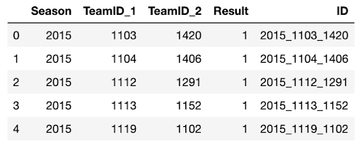
Next we got on with merging the engineered features onto both the test and training sets. The function works equally well for both the training and test sets, with the only difference being the first argument of the function:
- For the test set we used the output of the
prep_submission()function. - For the training set we used the output of the
prep_regseason()function.
def merge_features(features_df, ppg_df,eff_df,rankings_df):
    Wppg_df = ppg_df.rename(columns = {'PPG':'PPG_1','WPerc':'WPerc_1'})
    Lppg_df = ppg_df.rename(columns = {'PPG':'PPG_2','WPerc':'WPerc_2'})
    Wfeatures_df = pd.merge(features_df, Wppg_df,left_on=['Season', 'TeamID_1'], right_on=['Season', 'TeamID'], how='left')
    Wfeatures_df = Wfeatures_df.drop(['TeamID', 'GamesPlayed'], axis = 1)
    features_df = pd.merge(Wfeatures_df, Lppg_df,left_on=['Season', 'TeamID_2'], right_on=['Season', 'TeamID'], how='left')
    features_df = features_df.drop(['TeamID', 'GamesPlayed'], axis = 1)
    Weff_df = eff_df.rename(columns = {'oEFF': 'oEFF_1', 'dEFF': 'dEFF_1','oEFF_30day': 'oEFF_30day_1', 'dEFF_30day': 'dEFF_30day_1'})
    Leff_df = eff_df.rename(columns = {'oEFF': 'oEFF_2', 'dEFF': 'dEFF_2','oEFF_30day': 'oEFF_30day_2', 'dEFF_30day': 'dEFF_30day_2'})
    features_df = pd.merge(features_df, Weff_df, how = 'left', left_on = ['Season', 'TeamID_1'], right_on = ['Season', 'TeamID'])
    features_df = features_df.drop(['TeamID'], axis = 1)
    features_df = pd.merge(features_df, Leff_df, how = 'left', left_on = ['Season', 'TeamID_2'], right_on = ['Season', 'TeamID'])
    features_df = features_df.drop(['TeamID'], axis = 1)
    features_df['PPG_diff'] = features_df['PPG_1'] - features_df['PPG_2']
    features_df['WPerc_diff'] = features_df['WPerc_1'] - features_df['WPerc_2']
    features_df['oEFF_diff'] = features_df['oEFF_1'] - features_df['oEFF_2']
    features_df['dEFF_diff'] = features_df['dEFF_1'] - features_df['dEFF_2']
    features_df['oEFF_30day_diff'] = features_df['oEFF_30day_1'] - features_df['oEFF_30day_2']
    features_df['dEFF_30day_diff'] = features_df['dEFF_30day_1'] - features_df['dEFF_30day_2']
    features_df = features_df.drop(['PPG_1', 'WPerc_1', 'PPG_2', 'WPerc_2', 'oEFF_1', 'dEFF_1', 'oEFF_30day_1',
                                    'dEFF_30day_1', 'oEFF_2', 'dEFF_2', 'oEFF_30day_2', 'dEFF_30day_2'], axis = 1)
    Wrankings_df = rankings_df.rename(columns = {'MedianRank': 'MedianRank_1', 'MasseyRank': 'MasseyRank_1', 'MeanRank' : 'MeanRank_1'})
    Lrankings_df = rankings_df.rename(columns = {'MedianRank': 'MedianRank_2', 'MasseyRank': 'MasseyRank_2', 'MeanRank' : 'MeanRank_2'})
    features_df = pd.merge(features_df,Wrankings_df, how = 'left', left_on = ['Season', 'TeamID_1'], right_on = ['Season', 'TeamID'])
    features_df = features_df.drop(['TeamID'],axis = 1)
    features_df = pd.merge(features_df,Lrankings_df, how = 'left', left_on = ['Season', 'TeamID_2'], right_on = ['Season', 'TeamID'])
    features_df = features_df.drop(['TeamID'],axis = 1)
    features_df['MedianRank_diff'] = features_df['MedianRank_1'] - features_df['MedianRank_2']
    features_df['MasseyRank_diff'] = features_df['MasseyRank_1'] - features_df['MasseyRank_2']
    features_df['MeanRank_diff'] = features_df['MeanRank_1'] - features_df['MeanRank_2']
    features_df = features_df.drop(['MedianRank_1', 'MasseyRank_1', 'MeanRank_1',
                                    'MedianRank_2', 'MasseyRank_2', 'MeanRank_2'], axis = 1)
    return features_df
The first part of the function merged the points-per-game dataframe, the efficiency metrics dataframe, and the rankings dataframe onto the respective test or training dataframe. This implies two sets of metrics in each row: one for Team 1 and another for Team 2. To reduce the number of features, but still maintain the same amount of information, we were able to take the difference between each metric for each team. So, for example, the column PPG_diff contains the difference in PPG between Team 1 and Team 2. This is done for each feature.
The first few rows in our merged test set look like:

The first few rows in our merged training set look like:

Thus far, we have imported the data provided by the competition, and created functions for engineered features using this data. Now, we can move on to training the model.
Training & Testing the Model: 2015 to 2019 Regular Season
After writing all of the data manipulation functions, we can run the imported data through each one:
## prepare tournament submission df for 2015-2019, i.e. test set.
## Note: not all matchups have Results, as we predict all possible matchups (11,390) for the 5 seasons when only 335 games actually occur
features_df = prep_submission(ss_df,tcr_df)
ppg_df = get_ppg(rscr_df)
eff_df = get_efficiency(rsbs_df)
rankings_df = get_rank(massey_df)
tournament_df = merge_features(features_df, ppg_df,eff_df,rankings_df)
## prepare regular season df for 2015-2019, i.e. training set
rscr_df = prep_regseason(rscr_df)
regseason_df = merge_features(rscr_df, ppg_df,eff_df,rankings_df)
So, tournament_df contains our test data and regseason_df contains our training data.
Next, I split each set into each season. This step is more a matter of preference and is not absolutely necessary. I prefer to have different model parameters for each season than to group them all together. This gives insight on how the evaluation metric can change from year to year, given the same features (which is important for understanding the accuracy of our 2020 predictions); but also allows for different features to vary their importance from year to year. For instance, the Massey ranking could be an excellent predictor for one year, but not the next. If we were to combine all five seasons into a single model, this variability is not captured.
regseason_df_2015 = regseason_df[regseason_df.Season == 2015]
regseason_df_2016 = regseason_df[regseason_df.Season == 2016]
regseason_df_2017 = regseason_df[regseason_df.Season == 2017]
regseason_df_2018 = regseason_df[regseason_df.Season == 2018]
regseason_df_2019 = regseason_df[regseason_df.Season == 2019]
And we do the same for the test data:
## drop matchups that don’t occur, as we cannot evaluate them
tournament_df = tournament_df.dropna()
tournament_df_2015 = tournament_df[tournament_df.Season == 2015]
tournament_df_2016 = tournament_df[tournament_df.Season == 2016]
tournament_df_2017 = tournament_df[tournament_df.Season == 2017]
tournament_df_2018 = tournament_df[tournament_df.Season == 2018]
tournament_df_2019 = tournament_df[tournament_df.Season == 2019]
Now we split the datasets into a test and training set. I only included the 2015 season below, but the code is identical for the other seasons (just swap the year in the dataframe).
X_train = regseason_df_2015[['PPG_diff', 'WPerc_diff', 'oEFF_diff', 'dEFF_diff', 'oEFF_30day_diff',
                       'dEFF_30day_diff', 'MedianRank_diff', 'MasseyRank_diff', 'MeanRank_diff']]
y_train = regseason_df_2015[['Result']]
X_test = tournament_df_2015[['PPG_diff', 'WPerc_diff', 'oEFF_diff', 'dEFF_diff', 'oEFF_30day_diff',
                        'dEFF_30day_diff', 'MedianRank_diff', 'MasseyRank_diff', 'MeanRank_diff']]
y_test = tournament_df_2015[['Result']]
From here we can introduce a few different models. All of them will be some form of logistic regression, as we want to predict a binary variable: winning or losing. The metric that the competition uses to evaluate the predictions is known as log loss, so it makes sense to evaluate our model using the same metric. You can find out more about how log loss is calculated here.
The first model we can try is a plain old logistic regression:
from sklearn.linear_model import LogisticRegression
from sklearn.metrics import log_loss
clf = LogisticRegression(penalty='l1', dual=False, tol=0.001, C=1.0, fit_intercept=True,
                   intercept_scaling=1, class_weight='balanced', random_state=None,
                   solver='liblinear', max_iter=1000, multi_class='ovr', verbose=0)
#train and predict
clf.fit(X_train, np.ravel(y_train.values))
y_pred = clf.predict_proba(X_test)
y_pred = y_pred[:,1]
#log loss scoring
log_loss(y_test, y_pred, eps=1e-15, normalize=True, sample_weight=None, labels=None)
The log loss score I obtained was:
.05654409814609532
This serves as a base reference score with the given features we included in the training set. We can now use more advanced regressions to extract the most out of the features. For comparison, the previous competition winners for each season had scores of:
2015: 0.43893
2016: 0.48130
2017: 0.43857
2018: 0.53194
2019: 0.41477
Although not winning, we are within a reasonable range of log loss value on our first attempt. A more sophisticated model to attempt includes gradient boosting in the logistic regression model. To do so, we can use the xgboost package. Extreme gradient boosting is an algorithm that involves building multiple weak predictive models and iteratively minimizing a cost function (or in our case, the log loss) that results in a single strong predictive model. For a more in-depth discussion on the xgboost algorithm, see my article here. To implement this:
import xgboost as xgb
dtest = xgb.DMatrix(X_test, y_test, feature_names=X_test.columns)
dtrain = xgb.DMatrix(X_train, y_train,feature_names=X_train.columns)
param = {'verbosity':1,
         'objective':'binary:logistic',
         'booster':'gblinear',
         'eval_metric' :'logloss',
         'learning_rate': 0.05}
 evallist = [(dtrain, 'train')]
Feel free to adjust the learning rate or any of the other parameters to see how they affect the final log loss value.
num_round = 30
bst = xgb.train(param, dtrain, num_round, evallist)
The output displays the log loss value of the training set for each round. I obtained values of:
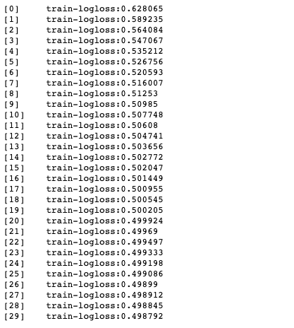
And for the test set:
0.5448100720323733
This is a bit better than using a single logistic regression model alone. As I mentioned previously, creating a model is an iterative process. Attempting different model parameters, removing/adding features, including alternative datasets, are all good practices to try before applying the model to the 2020 regular season data. I’ll leave these as exercises for the reader. Inspiration can be found on the competition Discussion board where other competitors share their own approaches, problems, models, and external data sources.
The Bracket that Could Have Been
The New York Post released their most probable bracket for the 2020 tournament, which can be seen below:
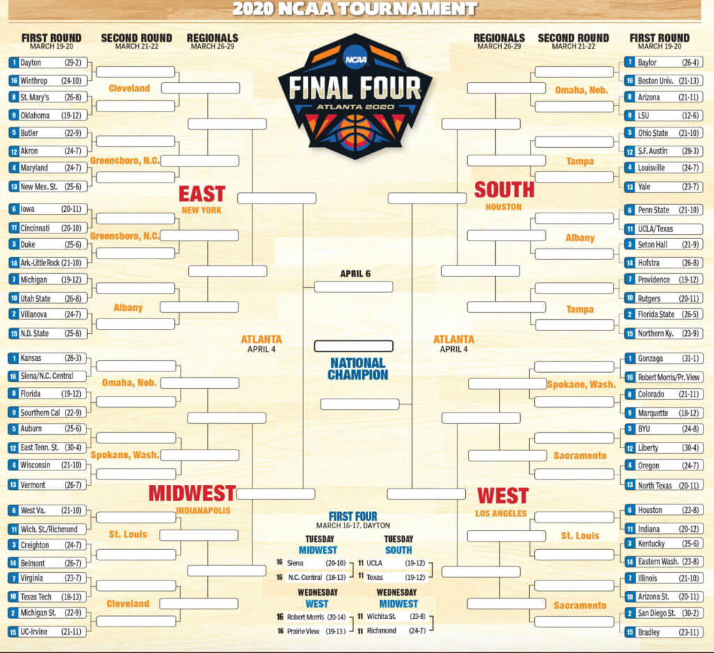
As an exercise for the reader, we can predict the win probabilities for each game in the first round. Of course, since Kaggle did not give us access to the 2020 dataset, the best we can do is use the 2019 data to predict for each team. For the First Four games, I assume the winners are Siena, Wichita State, UCLA, and Robert Morris. The first thing we do is create a list with the names of each of the first round matchups:
matchups = ['Dayton', 'Winthrop',
            "St Mary's CA", 'Oklahoma',
            'Butler', 'Akron',
            'Maryland', 'New Mexico St',
            'Iowa', 'Cincinnati',
            'Duke', 'Ark Little Rock',
            'Michigan', 'Utah St',
            'Villanova', 'N Dakota St',
            'Kansas', 'Siena',
            'Florida', 'USC',
            'Auburn', 'ETSU',
            'Wisconsin', 'Vermont',
            'West Virginia', 'Wichita St',
            'Creighton', 'Belmont',
            'Virginia', 'Texas Tech',
            'Michigan St', 'UC Irvine',
            'Baylor', 'Boston Univ',
            'Arizona', 'LSU',
            'Ohio St', 'SF Austin',
            'Louisville', 'Yale',
            'Penn St', 'UCLA',
            'Seton Hall', 'Hofstra',
            'Providence', 'Rutgers',
            'Florida St', 'N Kentucky',
            'Gonzaga', 'Robert Morris',
            'Colorado', 'Marquette',
            'BYU', 'Liberty',
            'Oregon', 'North Texas',
            'Houston', 'Indiana',
            'Kentucky', 'E Washington',
            'Illinois', 'Arizona St',
            'San Diego St', 'Bradley']
We can write a function to do all the processing we performed on all the other tournament data. The function looks like this:
def prep2020(matchups,teams_df,ppg_df,eff_df,rankings_df ):
    nyp_df = pd.DataFrame()
    for i in range(0,len(matchups),2):
        matchup_df = pd.DataFrame({'Team_1': matchups[i], 'Team_2': matchups[i+1]}, index = [i])
        nyp_df = pd.concat([nyp_df,matchup_df], axis = 0)
    nyp_df = pd.merge(teams_df[['TeamID','TeamName']],nyp_df,how = 'right', left_on = ['TeamName'], right_on = ['Team_1'])
    nyp_df = nyp_df.rename(columns = {'TeamID': 'TeamID_1'})
    nyp_df = nyp_df.drop(['TeamName', 'Team_1'], axis = 1)
    nyp_df = pd.merge(teams_df[['TeamID','TeamName']],nyp_df ,how = 'right', left_on = ['TeamName'], right_on = ['Team_2'])
    nyp_df = nyp_df.drop(['TeamName', 'Team_2'], axis = 1)
    nyp_df = nyp_df.rename(columns = {'TeamID': 'TeamID_2'})
    nyp_df['Season'] = 2019
    nyp_df['ID'] = nyp_df['Season'].astype(str) + '_' + nyp_df['TeamID_1'].astype(str) +'_' + nyp_df['TeamID_1'].astype(str)
    nyp_df = merge_features(nyp_df, ppg_df,eff_df,rankings_df)
    return nyp_df
The output looks similar to the other test sets for previous seasons:

And we can use models trained on the 2019 data to make predictions:
X_train = regseason_df_2019[['PPG_diff', 'WPerc_diff', 'oEFF_diff', 'dEFF_diff', 'tempo_diff', 'oEFF_30day_diff',
                       'dEFF_30day_diff','tempo_30day_diff', 'MedianRank_diff', 'MasseyRank_diff', 'MeanRank_diff']]
y_train = regseason_df_2019[['Result']]
X_test = nyp_df[['PPG_diff', 'WPerc_diff', 'oEFF_diff', 'dEFF_diff', 'tempo_diff', 'oEFF_30day_diff',
                       'dEFF_30day_diff','tempo_30day_diff', 'MedianRank_diff', 'MasseyRank_diff', 'MeanRank_diff']]
gbc = GradientBoostingClassifier(loss='deviance',
                             learning_rate=0.1,
                             n_estimators=100,
                             subsample=0.5,
                             criterion='friedman_mse',
                             min_samples_split=2,
                             min_samples_leaf=1,
                             min_weight_fraction_leaf=0.0,
                             max_depth=5,
                             max_features=None,
                             verbose=1,
                             max_leaf_nodes=None)
 gbc.fit(X_train, np.ravel(y_train.values))
y_pred = gbc.predict_proba(X_test)
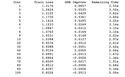
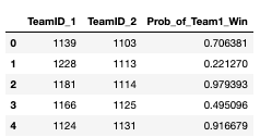
The first few predictions look like this:
nyp_df['Prob_of_Team1_Win'] = y_pred[:,1]
nyp_df[['TeamID_1', 'TeamID_2', 'Prob_of_Team1_Win']].head()
Summary
In this tutorial, we used Python to create an entry for the Google Cloud and NCAA March Madness competition with the goal of forecasting the outcome of the NCAA Division I Men’s Basketball Championship. While the championship and Kaggle competition were eventually cancelled for 2020, the steps illustrated in this post are just as valid for next year’s run. To reiterate:
- Choose a set of standard basketball statistics based on how they correlate with winning or losing.
- Extract these statistics from the data provided by Kaggle, and build your own features around them.
- Train different models for each of the last five seasons, and apply the best of these models to the current regular season data in order to make a set of predictions that can be submitted to the Kaggle competition.
I encourage all readers to try to improve their own models with additional model tuning and feature engineering. Once you do, take a look at the code in my repository to see where I made improvements as a point of comparison.
Congratulations! You’re all set to make your first entry to the March Madness competition when it reconvenes next year.
- All of the code used in this article can be found on my GitLab repository.
- Download the pre-built March Madness 2020 runtime environment for Windows 10, Linux or macOS and make your own predictions.


