Random Forest and XGBoost are two popular decision tree algorithms for machine learning. In this post I’ll take a look at how they each work, compare their features and discuss which use cases are best suited to each decision tree algorithm implementation. I’ll also demonstrate how to create a decision tree in Python using ActivePython by ActiveState, and compare two ensemble techniques, Random Forest bagging and extreme gradient boosting, that are based on decision tree learning. The code that I use in this article can be found here.
What is a decision tree algorithm?
Decision tree learning is a common type of machine learning algorithm. One of the advantages of the decision trees over other machine learning algorithms is how easy they make it to visualize data. At the same time, they offer significant versatility: they can be used for building both classification and regression predictive models.
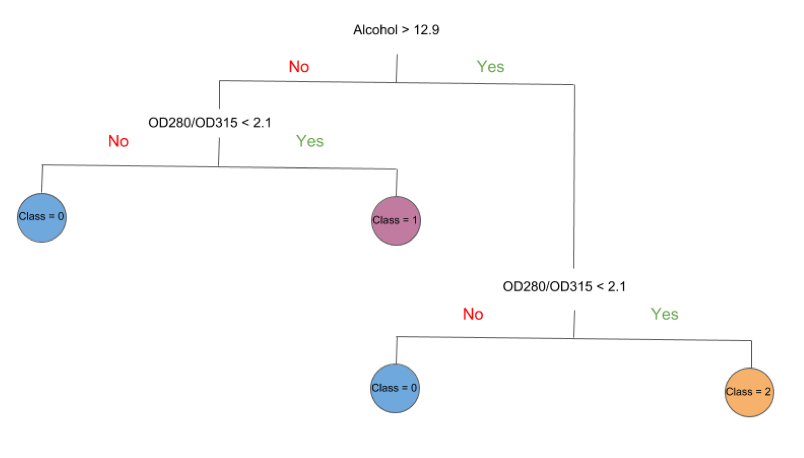
Decision tree algorithms work by constructing a “tree.” In this case, based on an Italian wine dataset, the tree is being used to classify different wines based on alcohol content (e.g., greater or less than 12.9%) and degree of dilution (e.g., an OD280/OD315 value greater or less than 2.1). Each branch (i.e., the vertical lines in figure 1 below) corresponds to a feature, and each leaf represents a target variable. In our case, the features are Alcohol and OD280/OD315, and the target variables are the Class of each observation (0,1 or 2).

As you can see, the tree is a simple and easy way to visualize the results of an algorithm, and understand how decisions are made. This elegant simplicity does not limit the powerful predictive ability of models based on decision trees. Without any fine tuning of the algorithm, decision trees produce moderately successful results. Coupled with ensemble methods that data scientists have developed, like boosting and bagging, they can achieve surprisingly high predictability.
A brief history may help with understanding how boosting and bagging came about:
- Tin Kam Ho first introduced random forest predictors in the mid-1990s. His paper elucidated an algorithm to improve the predictive power of decision trees: grow an ensemble of decision trees on the same dataset, and use them all to predict the target variable.
- Several years later, Jerome Friedman published a paper outlining another strategy for improving any predictive algorithm that he called generalized gradient “boosting,” which involves minimizing an arbitrary loss function. In the case of regression trees, the loss function weights each leaf within the tree differently, such that leaves that predict well are rewarded and those that do not are punished.
- Yet another strategy to improve decision tree models was developed by Leo Breiman in this paper. Commonly known as “bagging,” his technique creates an additional number of training sets by sampling uniformly and with replacement from the original training set.
Creating a Decision Tree
To implement the algorithm, I’ll be using the free community edition of ActivePython 3.6. Installation instructions can be found here.
The data we’ll use to build our model is from the UCI Machine Learning Repository. The wine dataset provides 178 clean observations of wine grown in the same region in Italy. Each observation is from one of three cultivars (represented as the ‘Class’ feature), with 13 constituent features that are the result of a chemical analysis.
import pandas as pd
import matplotlib.pyplot as plt
wine_names = ['Class', 'Alcohol', 'Malic acid', 'Ash', 'Alcalinity of ash', 'Magnesium', 'Total phenols', \
              'Flavanoids', 'Nonflavanoid phenols', 'Proanthocyanins', 'Color intensity', 'Hue', 'OD280/OD315',\
              'Proline']
wine_data = pd.read_csv('https://archive.ics.uci.edu/ml/machine-learning-databases/wine/wine.data', names = wine_names)
wine_df = pd.DataFrame(wine_data)
wine_df.Class = wine_df.Class - 1
After importing the pandas library and the wine dataset, I converted the dataset to a pandas DataFrame. To create the decision tree, I used the DecisionTreeClassifier within the scikit-learn package (refer to the documentation for further information). It is also necessary to split the dataset into a test and training set in order to properly evaluate each of the different models:
from sklearn.model_selection import train_test_split
Y = wine_df.loc[:,'Class'].values
X = wine_df.loc[:,'Alcohol':'Proline'].values
#we split the dataset into a test and training set
train_x, test_x, train_y, test_y = train_test_split(X,Y , test_size=0.3, random_state=0)
from sklearn import tree
clf = tree.DecisionTreeClassifier(max_depth=2)
clf = clf.fit(train_x, train_y)
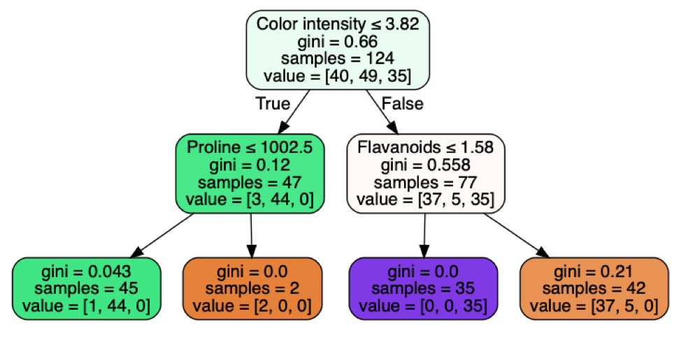
The tree created with the training set looks like this:

The bottom row consists of the “leaves” of the decision tree. The purity of each leaf is characterized by the Gini index: the closer to 0, the purer the leaf. For example, the first leaf correctly predicts the class for 44 of the 45 samples that satisfies the inequalities of the first and second branches (Color intensity and Proline). I’ve limited the tree depth to two levels for simplicity, but even with this limitation, the model predicts the correct class ~87% of the time in the test set.
ftest_score = clf.score(test_x, test_y)
test_score

This result is great, but by using the techniques proposed by Ho, Breiman and Friedman, we can improve the performance of the model.
Feature & Tree Bagging
To implement Random Forest, I imported the RandomForestClassifier:
from sklearn.ensemble import RandomForestClassifier
RF_clf = RandomForestClassifier(n_estimators=100, max_depth=2, max_features = 'sqrt',verbose = 1, bootstrap = False)
RF_clf.fit(train_x, train_y)
I used the default number of decision trees (100) and the maximum number of features in each tree to the square root of the total number of features. You can refer to Breiman’s paper for his reasoning for using the square root, but it generally is the best choice in all cases to minimize the variance. I maintained the max depth at 2, for consistency.
test_score = RF_clf.score(test_x, test_y)
test_score

By introducing bagging into the model, I achieved a ~10% increase in the number of correctly predicted classes.
Gradient Descent Boosting
To implement gradient descent boosting, I used the XGBoost package developed by Tianqi Chen and Carlos Guestrin. They outline the capabilities of XGBoost in this paper. The package is highly scalable to larger datasets, optimized for extremely efficient computational performance, and handles sparse data with a novel approach. Due to the nature of the dataset I use in this article, these benefits may manifest, but must be considered when implemented on a much larger scale. To start, I imported the package, prepared the test and training data, and the parameters of the model:
import XGBoost as xgb
from sklearn.metrics import accuracy_score
dtest = xgb.DMatrix(test_x, test_y, feature_names=wine_names[1:14])
dtrain = xgb.DMatrix(train_x, train_y,feature_names=wine_names[1:14])
param = {'max_depth': 2,
         'learning_rate': 0.3,
         'verbosity': 1,
         'objective': 'multi:softmax',
         'num_class': 3,
         'eval_metric': 'merror'}
		 evallist = [(dtrain, 'train')]
We can then train the model, specifying the number of iterations to minimize the loss function:
num_round = 10
bst = xgb.train(param, dtrain, num_round, evallist)

Setting the verbosity to 1 allows us to see the loss function minimized at each step. Next, we can test the model to achieve a similar increase in the number of correctly predicted classes:
ypred = bst.predict(dtest, ntree_limit=bst.best_ntree_limit)
accuracy_score(test_y,ypred)

Conclusion
To summarize, bagging and boosting are two ensemble techniques that can strengthen models based on decision trees. Using Random Forest generates many trees, each with leaves of equal weight within the model, in order to obtain higher accuracy. On the other hand, Gradient Descent Boosting introduces leaf weighting to penalize those that do not improve the model predictability. Both decision tree algorithms generally decrease the variance, while boosting also improves the bias.
- To view all the code and data mentioned in this post, you can refer to my Gitlab repository.
- To run the code, you can sign up for a free ActiveState Platform account and either build your own runtime environment or download the pre-built ActivePython runtime.
Title photo courtesy of alt-free-download.com.


