In this blog: Understand how Python can be used to solve some of the most common problems encountered by scientists and researchers. Download the Scientific Computing runtime environment and start learning more about what Python can do for you.
How useful is Python for scientists? If you are a scientist or a researcher asking this question then you’ve stumbled upon the right blog. You must find yourself wasting a lot of time doing menial tasks within the context of analysis or figure creation, or just in trying to bridge the gap between simulation software. We will show you how Python can resolve these issues with ease. Although we will be using a specific simulation package as an example, the code is general and simple enough for you to apply to your own use case.
The increasing popularity of Python among data scientists and developers within the software industry has begun to spill over into the slow-moving behemoth that is academia. Despite being at the forefront of fundamental science and engineering research, the members of academia themselves are too often entrenched in the methodologies and legacy languages they learned when they first started their careers. As the turnover in programming languages outpaces that of academic careers, this can lead to procedural inefficiencies that result in wasted time, money, and other precious resources. Fortunately, Python is here to save the day.
The versatility, ease of use, and readability of Python lower the learning curve such that even the most entrenched academics can adopt it. In all areas of research, from statistics to material science, Python can help bridge the procedural gaps that would otherwise be carried out with other inefficient alternatives such as spreadsheets, text editors, or even manual processes carried out by hand.
Through an example of the simple task automating file conversion, we are going to demonstrate the use of Python for science and research. Let’s start with installing Python for scientists and researchers.
Installing Python for science and computing
To follow along with the code in this article, you can get our “Scientific Computing” runtime environment for Windows, macOS, or Linux, which contains a version of Python and all of the packages used in this post. The easiest way to get it is to do the following:
- Create a free ActiveState Platform account
- Install the “Scientific Computing” build
NOTE: the simplest way to install the Scientific Computing runtime is to first install the ActiveState Platform’s command-line interface (CLI), the State Tool.
- If you’re on Windows, you can use Powershell to install the State Tool:
IEX(New-Object Net.WebClient).downloadString('https://platform.www.activestate.com/dl/cli/install.ps1')
- If you’re on Linux / Mac, you can use curl to install the State Tool:
sh <(curl -q https://platform.www.activestate.com/dl/cli/install.sh)
Once the State Tool is installed, just run the following command to download the build and automatically install it into a virtual environment:state activate Pizza-Team/Scientific-Computing
All of the code and files used in this article can be found in our GitLab repository.
All set? Let’s go.
Python for Scientists and Researchers: How to Convert Between File Formats Using Python
A common obstacle in academia is the incompatibility between the file types of different programs. Typically, the information that is output by one program is used as an input for another, but the file structure may not be readable by the other program. Automating file conversion is a common task for Python, allowing you to perform conversions instantly on any number of files.
The following code converts a file that geometrically defines a crystal structure (in the form of a .vasp file) into a LAMMPS configuration file. LAMMPS is the file format for a molecular dynamics simulation program. Note that the exact types of files and programs are not important. What is important is that both types of files can be opened and read by a text editor, and that conversion with Python is instantaneous.
First, we define the filename and import and export paths:
fileName = 'liquid_configuration_CuZr'
importPath = './input-files/' + fileName + '.POSCAR.vasp'
exportPath = './generated-data/' + fileName + '.lammps'
Then, we open the file and read through each line:
lines = open(importPath,'r').readlines()
Lines 2-4 of our file tell us the size of the simulation box, which can be read as the following diagonal matrix:

To save this simulation box size information, we can do the following:
matrix = {}
matrix['x'] = float(lines[2].split()[0])
matrix['y'] = float(lines[3].split()[1])
matrix['z'] = float(lines[4].split()[2])
The code splits each line (corresponding to each dimension) into a list of strings, converts them to a numerical float, and assigns the float to the matrix diagonal element.
- Atom type
- Number of atoms
- Atomic weight
elements = lines[5].split()
counts = [int(x) for x in lines[6].split()]
atomsPresent = {}
for i in range(len(elements)):
    key = elements[i]
    atomsPresent[key] = {}
    atomsPresent[key]['atomType'] = i+1
    atomsPresent[key]['counts'] = counts[i]
    atomsPresent[key]['mass'] = atomic_weight[key]
print(atomsPresent)
You should see an output like this:
{'Cu': {'atomType': 1, 'counts': 1500, 'mass': 63.546}, 'Zr': {atomType': 2, 'counts': 1500, 'mass': 91.224}}
Line 8 of a .vasp file is the beginning of the atomic coordinates. Each line has extra white spaces, so for each one, we will:
- Split the string into a list of strings
- Join them with a single whitespace
- Add the three zeroes for the image flags to the string with a single whitespace.
coordinates = []
for i in range(8,len(lines)):
    coordinates.append(' '.join(lines[i].split()) + ' 0 0 0 \n')
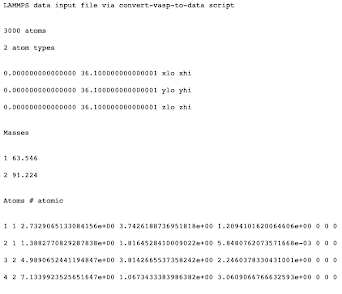
We now have all of the relevant information needed for the .lammps import file. The format of the import file must look similar to:

To create this structure in Python, we use the write method and loop over the atomsPresent dictionary:
f = open(exportPath,'w')
f.write('LAMMPS data input file via convert-vasp-to-data script\n\n')
f.write('%d atoms\n' % (len(coordinates)))
f.write('%d atom types\n\n' % (len(atomsPresent)))
f.write('%1.15f %1.15f xlo xhi\n' % (0,matrix['x']))
f.write('%1.15f %1.15f ylo yhi\n' % (0,matrix['y']))
f.write('%1.15f %1.15f zlo zhi\n\n' % (0,matrix['z']))
f.write('Masses\n\n')
for i in range(len(atomsPresent)):
    f.write('%d %1.3f\n' % (atomsPresent[elements[i]]['atomType'],atomsPresent[elements[i]]['mass']))

index = 0
atomID = 1
f.write('\nAtoms # atomic\n\n')
for i in range(len(atomsPresent)):
    key = elements[i]
    for j in range(atomsPresent[key]['counts']):
        f.write('%d %d ' % (atomID, atomsPresent[key]['atomType']) + coordinates[index])
        index += 1
        atomID += 1
f.close()
print('File has been printed to: ',exportPath)
After running the code, we should see a message like:
File has been printed to: ./generated-data/liquid_configuration_CuZr.lammps
If you open the export path location on your system, you should now see the new file.
Python for Scientists and Researchers: How to Analyze and Plot Data Using Python
Another common problem encountered by scientists and researchers is efficiently analyzing raw data from a program and creating meaningful figures with the data. Python can be used to efficiently loop through any number of output data files and produce journal-quality figures on the fly.
For this example, we will use the raw output file produced by the LAMMPS simulation software. The output file contains the information and results for a given simulation. First, we read the file:
fileName = './input-files/log-1.lammps'
lines = open(fileName,'r').readlines()
In order to efficiently interpret the data and put it in the right format, Python’s pandas dataframe feature comes in handy. Pandas is a Python package specifically designed for data manipulation. Using pandas, we can loop through each line and assign each property of interest (step, temperature, potential energy, total energy, pressure, and volume) to a column. Each row will correspond to a time step (i.e. the Step property).
import pandas as pd
data = []
for i in range(len(lines)):
    if "Per MPI rank memory allocation (min/avg/max) =" in lines[i]:
        header = lines[i+1].split()
        placer = i+2
        while 'Loop time of ' not in lines[placer]:
            data.append([float(value) for value in lines[placer].split()])
            placer += 1
data = pd.DataFrame(data, columns = header)
data.head()

Thus far, our code only deals with a single output file, but we can generalize it to handle any number of files. The best way to do this is by reformulating the operations into a single function, and then running each file through that function in a loop:
def returnLAMMPSdata(filePath):
    lines = open(filePath,'r').readlines()
    data = []
    for i in range(len(lines)):
        if "Per MPI rank memory allocation (min/avg/max) =" in lines[i]:
            header = lines[i+1].split()
            placer = i+2
            while 'Loop time of ' not in lines[placer]:
                data.append([float(value) for value in lines[placer].split()])
                placer += 1
    data = pd.DataFrame(data, columns = header)
    return data
log1 = returnLAMMPSdata('input-files/log-1.lammps')
log2 = returnLAMMPSdata('input-files/log-2.lammps')
log3 = returnLAMMPSdata('input-files/log-3.lammps')
log4 = returnLAMMPSdata('input-files/log-4.lammps')
log4.head(5)

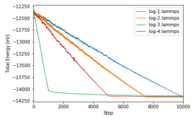
The output is a table that’s a little hard to read. Better would be if we could plot the results on a graph. Python’s matplotlib package can help us do just that:
import matplotlib.pyplot as plt
%matplotlib inline
plt.figure()
plt.plot(log1.Step,log1.TotEng, linewidth = 1, label = 'log-1.lammps')
plt.plot(log2.Step,log2.TotEng, linewidth = 1, label = 'log-2.lammps')
plt.plot(log3.Step,log3.TotEng, linewidth = 1, label = 'log-3.lammps')
plt.plot(log4.Step,log4.TotEng, linewidth = 1, label = 'log-4.lammps')
plt.xlim(0,10000)
plt.xlabel('Step')
plt.ylabel('Total Energy [eV]')
plt.legend()
plt.show()

In this way, a journal-worthy figure can be produced with ease, plotting data from multiple different files.
Summary
In this article, we used Python to solve some of the most common problems encountered by scientists and researchers across academia. Python is easy to learn, even without any prior programming experience. Using it to automate common tasks can save time, money, and other vital academic resources by replacing manually-executed processes typically done by hand with a far more efficient mechanism.
- For a more detailed description of the code as well as the code itself, check out this GitLab repository.
- Sign up for a free ActiveState Platform account so that you can download the Scientific Computing runtime environment and start learning more about what Python can do for you.
Related Blogs:


