In this article, I’ll introduce you to ten Pandas functions that will make your life easier (in no particular order), as well as provide some code snippets to show you how to use them. I’ll be applying the Pandas functions to a Pokemon dataset, so let’s dive into our pokedex!
Before you start: Install Python & Pandas
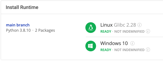
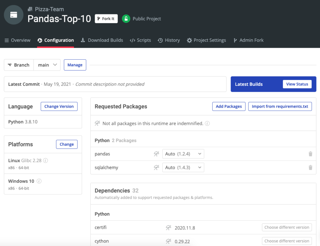
To follow along, you can install the Pandas Top 10 environment for Windows or Linux, which contains Python 3.8 and Pandas
In order to download this ready-to-use Python environment, you will need to create an ActiveState Platform account. Just use your GitHub credentials or your email address to register. Signing up is easy and it unlocks the ActiveState Platform’s many benefits for you!
Or you could also use our State tool to install this runtime environment.
For Windows users, run the following at a CMD prompt to automatically download and install our CLI, the State Tool along with the Pandas Top 10 runtime into a virtual environment:
powershell -Command "& $([scriptblock]::Create((New-Object Net.WebClient).DownloadString('https://platform.www.activestate.com/dl/cli/install.ps1'))) -activate-default Pizza-Team/Pandas-Top-10"
For Linux users, run the following to automatically download and install our CLI, the State Tool along with the Pandas Top 10 runtime into a virtual environment:
sh <(curl -q https://platform.www.activestate.com/dl/cli/install.sh) --activate-default Pizza-Team/Pandas-Top-10
1–The Read_X Family Functions
Your first task is usually to load the data for analysis, and Pandas offers a large family of functions that can read many different data formats. CSV files are the most common, but Pandas also supports many other formats, including:
- Microsoft Excel
- Fixed-width formatted lines
- Clipboard (it supports the same arguments as the CSV reader)
- JavaScript Object Notation (JSON)
- Hierarchical Data Format (HDF)
- Column-oriented data storage formats like Parquet and CRC
- Statistical analysis packages like SPSS and Stata
- Google’s BigQuery Connections
- SQL databases
To load data from databases, you can use the SQLAlchemy package, which lets you work with a huge number of SQL databases including PostgreSQL, SQLite, MySQL, SAP, Oracle, Microsoft SQLServer, and many others.
In the following example, a JSON file is loaded as a DataFrame:
import pandas as pd
df = pd.read_json('./pokedex.json')
df.head()
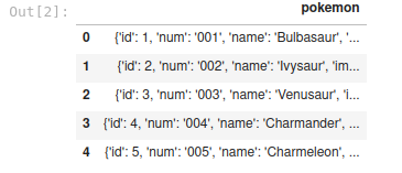
The read_x family of functions is very robust and flexible. However, that doesn’t mean you always get what you want with no effort. In this example, you can see that the pokemon column is fully loaded as individual rows, which is not very useful. Pandas includes another function that will allow you to make more use of this information.
2–The Json_Normalize Function
You can use the json_normalize function to process each element of the pokemon array and split it into several columns. Since the first argument is a valid JSON structure, you can pass the DataFrame column or the json parsed from the file. The record_path argument indicates that each row corresponds to an element of the array:
fObj = open("./pokedex.json")
jlist = json.load(fObj)
df = pd.json_normalize(jlist, record_path=['pokemon'])
df.head()
Meta and record_path give this function great flexibility, but not enough to process json without a unified structure. If you try to process the next_evolution or prev_evolution columns in the same way, you’ll get an error even if you use the errors=’ignore’ argument:
df = pd.json_normalize(jlist['pokemon'], record_path='next_evolution', meta=['id','name'], errors='ignore')
df.head()
---------------------------------------------------------------------------
KeyError                                  Traceback (most recent call last)
<ipython-input-20-b9ae9df69b00> in <module>
----> 1 df = pd.json_normalize(jlist['pokemon'], record_path='next_evolution', meta=['id','name'], errors='ignore')
     2 df.head()
~/.virtualenvs/fixate/lib/python3.8/site-packages/pandas/io/json/_normalize.py in _json_normalize(data, record_path, meta, meta_prefix, record_prefix, errors, sep, max_level)
   334                 records.extend(recs)
   335
--> 336     _recursive_extract(data, record_path, {}, level=0)
   337
   338     result = DataFrame(records)
~/.virtualenvs/fixate/lib/python3.8/site-packages/pandas/io/json/_normalize.py in _recursive_extract(data, path, seen_meta, level)
   307         else:
   308             for obj in data:
--> 309                 recs = _pull_records(obj, path[0])
   310                 recs = [
   311                     nested_to_record(r, sep=sep, max_level=max_level)
~/.virtualenvs/fixate/lib/python3.8/site-packages/pandas/io/json/_normalize.py in _pull_records(js, spec)
--> 248         result = _pull_field(js, spec)
   249
   250         # GH 31507 GH 30145, GH 26284 if result is not list, raise TypeError if not
~/.virtualenvs/fixate/lib/python3.8/site-packages/pandas/io/json/_normalize.py in _pull_field(js, spec)
   237                 result = result[field]
   238         else:
--> 239             result = result[spec]
   240         return result
   241
KeyError: 'next_evolution'
The problem is twofold:
- Not all pokemon have a next_evolution attribute
- The errors=’ignore’ argument only applies to the columns defined in the meta list
To process the lists of values and nested structures, you’ll need to use another approach.
3–The Explode Function
You will notice that there are some columns (type, multipliers, and weaknesses) in the DataFrame that contain lists of values. You can expand those values to new rows using the explode function, which will replicate the row data for each value in the list:
df = df.explode('weaknesses')
df.head()
As you can see, the index is repeated for Bulbasaur along with the other values (except weaknesses). However, the explode function won’t help you if you want new columns instead of new rows. In that case, you will have to write a function to process the values and return new columns.
4–The Apply Function
One of the most important functions of Pandas (which all data analysts should be proficient with) is the apply function. It allows you to work with the rows or columns of a DataFrame, and you can also use lambda expressions or functions to transform data.
Here’s how you expand the weaknesses, next_evolution, and prev_evolution columns using apply:
def get_nums(x):
   try:
       iterator = iter(x)
   except TypeError:
       return None
   else:
       return [c['num'] for c in x]
fObj = open("./pokedex.json")
jlist = json.load(fObj)
df = pd.json_normalize(jlist, record_path=['pokemon'])
df['evolutions'] = df['next_evolution'].apply( lambda x: get_nums(x) )
df['ancestors'] = df['prev_evolution'].apply( lambda x: get_nums(x) )
weaknesses = df['weaknesses'].apply( pd.Series )
evolutions = df['evolutions'].apply( pd.Series )
ancestors = df['ancestors'].apply( pd.Series )
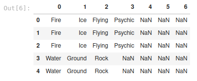
weaknesses.head()
The get_nums function checks to see if the cell value passed as an argument and if it’s iterable. If so, it will extract the values of the num keys and return them as a list. Then, the apply function will split the values from the list as columns and transform them into a Pandas Series. This will result in three new DataFrames that should be connected to the main DataFrame.
5–The Rename Function
It’s a good idea to rename the columns before merging the results from the previous operation with the main DataFrame, because default names like 1, 2, or n can get confusing and cause problems. The rename function can also be used with indexes, and it can take either a list or a function as an argument:
weaknesses = weaknesses.rename(columns = lambda x: 'wk_' + str(x))
evolutions = evolutions.rename(columns = lambda x: 'ev_' + str(x))
ancestors = ancestors.rename(columns = lambda x: 'an_' + str(x))
weaknesses.head()
6–The Merge Function
At this point, we have four separate DataFrames, but it’s usually better to have just one. You can combine DataFrames using the merge function, which works a lot like the database’s join operation. For example, you can join DataFrames A and B based on a specific type of combination (inner, left, right, outer, and cross) to create DataFrame C. In this case, since the DataFrames contain the same indexes, the inner option is the appropriate choice for a horizontal concatenation:
df = df.merge(weaknesses, left_index=True, right_index=True).merge(evolutions, left_index=True, right_index=True).merge(ancestors, left_index=True, right_index=True)
df.head()
The results show that columns wk_0 to wk_6, ev_0 to ev_2, and an_0 to an_1 were merged to the main DataFrame. Merge is flexible enough that it can be used with specific columns as well as indexes. You can also rename the overlapping columns on the fly and automatically validate the operation in case there are one-to-many or many-to-many cases that are not compatible with the type of merge that you are trying to apply.
7–The Iloc Function
Once you’ve completed the basic transformations, you often have to navigate through the data to get to specific slices that might be useful. The first way to do this is with the iloc function, which returns segments based on the index of the DataFrame:
_evens = df.iloc[lambda x: x.index % 2 == 0]
_evens.head()
In this example, we selected the even rows from the DataFrame using a simple lambda expression. Iloc is also flexible, allowing you to pass a specific index, a range of integers, or even slices. Here, we selected two rows and three columns:
df.iloc[1:3, 0:3]
This is usually the fastest way to extract subsets of a DataFrame, but it can also be accomplished by selecting information based on labels instead of positions.
8–The Loc Function
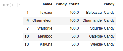
To select information based on labels, you can use the loc function. Below, we used a conditional over the values of the column candy_count to select a subset and return three columns:
slice_candies = df.loc[lambda df: df['candy_count'] > 30, ['name', 'candy_count', 'candy']]
slice_candies.head()
The power of the loc function is that you can combine complex selection criteria over the DataFrame. Another advantage of loc is that it can be used to set values for the resulting subset. For example, we can set the value of the rows without candy_count to zero using the following code:
df.loc[lambda df: np.isnan(df['candy_count']), ['candy_count']] = 0
df.head()
9–The Query Function
Another way to select a subset of data from a DataFrame is to use the query function, which allows you to operate over columns and refer to external variables in the query definition. Here is what it looks like when you select even rows that contain an above-average candy_count:
mean_candy_count = df['candy_count'].mean()
df.query('(index %2 == 0) and (candy_count > @mean_candy_count)').head()
The query function can even filter the DataFrame in which it is operating, meaning that the original DataFrame will be replaced with the results of the query function. It uses a slightly modified Python syntax, so be sure that you understand the differences before using it.
10–The Sample Function
The sample function will return a random sample from the DataFrame. You can parametrize its behavior by specifying a number of samples to return, or a specific fraction of the total required. The replace flag will allow you to select the same row twice, and the random_state argument will let you use a random seed for reproducible results. By default, every row has the same probability of being selected in the sample, but you can modify this with the weights argument.
samples = df.sample(frac=0.3, replace=True, random_state=42)
samples.head()
Proficiency with Pandas is simply one of those must learn Python skills for any developer.
Pandas is one of the most comprehensive tools you’ll ever use in Python. It’s fast, consistent, and fully charged with robust functions. We’ve covered ten of the most important Pandas functions in this article, but the list could be expanded to include further functions like plotting, indexing, categorizing, grouping, windowing, and many more.
Put your skills to use: Here’s a pre-compiled Pandas Python environment and the GitHub source code related to this post!
- You can find all of the code that we used in this article on GitHub.
- You can sharpen your Pandas skills by installing the Pandas Top 10 runtime environment and trying out the top 10 functions for yourself.
With the ActiveState Platform, you can create your Python environment in minutes, just like the one we built for this project. Try it out for yourself or learn more about how it helps Python developers be more productive.
*Hero banner image source: inprogresspokemon.tumblr.com/post/155399033729/6745-pancham-have-a-lot-of-attitude-for-such
Related Reads
Will AI Save Us? Use this Pandas Data Analysis Tutorial to find out.


