If you work with data, especially relational data, the Structured Query Language (SQL) is your lingua franca. Without a doubt, SQL is one of the most useful languages for any programmer to learn. It’s the language we use to communicate with the most commonly deployed database systems, including MySQL, PostgreSQL and Oracle. SQL has been the standard database query language for the past 50 years because it is both expressive and easy to use.

Be forewarned, though, that not all data structures support simple queries. The complexity of a query increases with the normalization level of the dataset. For example, with low-normalized (1-2 NF) datasets, all the data can be accessed with a simple SELECT statement. But with higher normalization levels (3NF, BCNF), the data are divided into multiple tables, which means you’ll need to use multiple JOIN statements to combine datasets before creating your query. 

While it will take quite a few practice sessions before you’ll be able to perform efficient queries, there are some top commands that you’ll find yourself using over and over. They also tend to be the most useful. 

This blog post will provide you with a good grounding of how to use the top 10 SQL commands against a public movie rental dataset. 

To follow along with this post, you’ll need to download and install the following:

• A copy of pgadmin from pgadmin.org
• A copy of the PostgreSQL database, which comes with the psql tool

All set? Let’s get started.

Create a PostgreSQL Dataset

Before we can start practicing SQL queries, we’ll need a database to query against. In this case, we’ll create a PostgreSQL database from publicly available movie rental data using pgadmin for easier SQL administration and query execution. 

Step 1 – Create the database by executing the following query:

CREATE DATABASE pagila
    WITH 
    OWNER = postgres
    ENCODING = 'UTF8'
    CONNECTION LIMIT = -1;

Here we can see first hand the CREATE DATABASE command, which is used to create a database with a provided name.

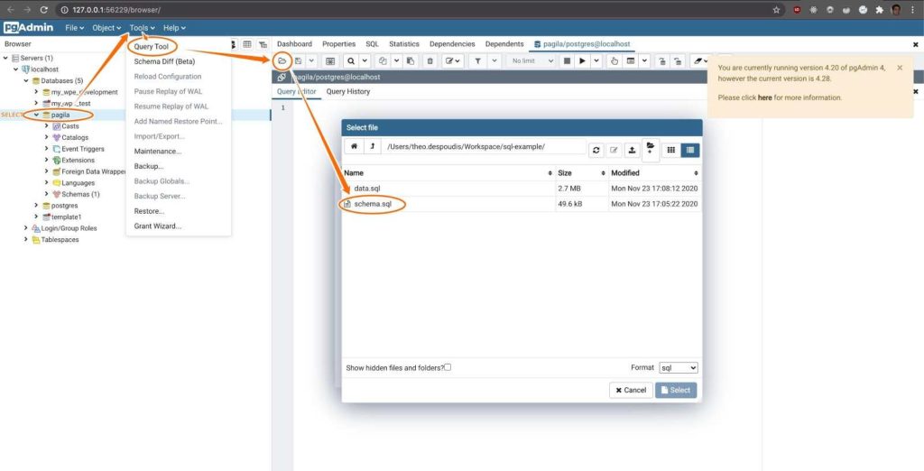
Step 2 – Create the schema by downloading the schema definition and executing it with the query tool options:

$ curl https://raw.githubusercontent.com/morenoh149/postgresDBSamples/master/pagila-0.10.1/pagila-schema.sql --output schema.sql

Once loaded in pgadmin, we can use the UI to execute the script by clicking on the right-pointing forward arrow or by pressing F5.

Step 3 – Load the data into the database. Download the data using the curl tool, and insert it into the database using the psql tool:

$ curl https://raw.githubusercontent.com/morenoh149/postgresDBSamples/master/pagila-0.10.1/pagila-data.sql --output data.sql
$ psql -d pagila -f data.sql

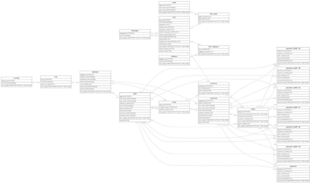
Once loaded, we can use the pgAdmin UI to inspect the dataset tables. Here is an Entity Relationship Diagram (ERD) of the database, showing how each element in the database is related:

Top 10 SQL Commands

Before delving into the examples, it’s important to understand the two different language groups that databases accept:

• DDL or Data Definition Language is a set of commands that describe the schema of the database in terms of tables, constraints or sequences. 
  • For example, these include the CREATE DATABASE command that we used in this post, but also the INSERT INTO command used to insert data into a table, as well as the UPDATE command, which is used to update data.
• DML or Data Manipulation Language is a set of commands that allow us to query the state of the database. 
  • DML contains all of our top 10 SQL commands.

#1 — SELECT

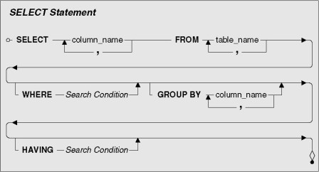
The SELECT statement is the bread and butter of SQL DML because the majority of all commands start with this operator. We can use it for selecting individual columns or rows from a table, or just for evaluating expressions. Here are some examples from the dataset:

• Select all fields from the customer table

SELECT * FROM customer;

• Select only the title description and year fields from the film table

SELECT title, description, release_year from film; 

• Calculate the sum of all rental sales using the payment table

SELECT SUM(amount) from payment;

• Print the current datetime

SELECT now();

#2 — WHERE

When we want to limit or filter the SELECT statement results based on some condition, we need to use the WHERE command. Here are some examples from the dataset:

• Select all payments worth more than $5

SELECT * from payment where amount > 5;

• Select all customers where their surname is ‘smith’

SELECT * from customer where LOWER(last_name)= 'smith';

• Select all film rentals that occurred on the date 2005-05-24

SELECT * FROM rental WHERE DATE(rental_date)='2005-05-24'

#3 — BETWEEN

When we want to select values within a range, we use the BETWEEN command. We need to provide a starting point and an endpoint using the WHERE operator:

• Select all rentals that occurred between 2005-05-24 and 2005-05-30

SELECT * FROM rental WHERE DATE(rental_date) BETWEEN '2005-05-24' AND '2005-05-30';

#4 — AND/OR/NOT

AND, OR and NOT are boolean operators. They allow us to apply boolean algebra in order to filter our results. For example:

• Select all rentals with a specific inventory_id and a specific customer_id

SELECT * FROM rental WHERE inventory_id=1525 AND customer_id=127;

• Select all rentals that occurred on either 2005-05-24 or 2005-05-30

SELECT * FROM rental WHERE DATE(rental_date)='2005-05-24'OR DATE(rental_date)='2005-05-30';

• Select all films that were released in 2006 but did not have an NC-17 rating

SELECT * FROM film WHERE release_year=2006 AND NOT rating='NC-17';

#5 — MIN/MAX

When we need to find the maximum or the minimum value in a column, we use the MIN/MAX functions. For example:

• Select the maximum and minimum replacement costs from the film table

SELECT MAX(replacement_cost), MIN(replacement_cost) FROM film;

#6 — LIMIT/OFFSET

When we want to restrict the number of results, or else implement paginated results (starting from a different position other than the initial one), we use the LIMIT and OFFSET operators:

• Select the first ten payment details after the first fifty results

SELECT * FROM payment ORDER BY payment_date DESC LIMIT 10 OFFSET 50;

#7 — IN

The IN operator is used for checking inclusion criteria. For example, we can check which of the results exist in the list of values to test. Here is an example query:

• Select all films that have the same maximum replacement cost

SELECT film_id, title, replacement_cost FROM film WHERE replacement_cost IN (SELECT MAX(replacement_cost) FROM film)

#8 — ORDER BY/GROUP BY

When we want to order our results in an ascending or descending order, we can use the ORDER BY clause. We can use GROUP BY to create aggregate columns by calculating some value from all the rows in a table.

• Select all films and order them in descending order of film length (from the longest to the shortest)

SELECT * from film ORDER BY length DESC;

• Select each date and the total amount of all payments made on that date from the payment table

SELECT DATE(payment_date), SUM(amount) from payment GROUP BY DATE(payment_date);

• Select each date and the total amount of payments made on that date from the payment table, and then order them in descending order

SELECT DATE(payment_date) as PaymentDate, SUM(amount) as Total from payment GROUP BY PaymentDate ORDER BY Total DESC;

#9 — HAVING

If we want to filter Aggregate functions such as SUM or AVG that result from the use of a GROUP BY command, we need to use the HAVING operator because WHERE is cannot be used with aggregate functions:

• Select each date and the total amount of all payments made on that date from the payment table, but print only the ones worth more than $3000 in total

SELECT DATE(payment_date) as PaymentDate, SUM(amount) as total from payment GROUP BY PaymentDate HAVING SUM(amount) > 3000;

• Select the number of films, their rating and their average replacement cost, but print only the ones that have an average replacement cost of less than $19

SELECT COUNT(film_id), rating, AVG(replacement_cost) as AvgReplacementCost from film GROUP BY rating HAVING AVG(replacement_cost) < 19;

#10 — INNER JOIN

If SELECT is the bread and butter of SQL commands, then JOINing tables is the salt and pepper. We need to use JOINs to combine table relationships together and create common datasets.

• Show the actor and film details together in one table.

SELECT first_name, last_name, title, description FROM film_actor fa INNER JOIN actor ON (fa.actor_id = actor.actor_id) INNER JOIN film on (fa.film_id = film.film_id);

The film has a many-to-many relationship with the actor, so we use the film_actor table as a joining point. We JOIN film_actor and actor together and then we JOIN film_actor and film together. The SELECT operator will now have access to all columns from the two tables.

SQL commands within a programming language like Python

There are many more SQL commands available in modern database systems, including INSERT, LIKE, DELETE FULL OUTER JOIN, COUNT, AS, and DROP. Some specialized databases will even have their own specialized commands, such as those for Geographic Information Systems (GIS), which include functions like ST_contains or ST_covers for geometrical queries.

But once you have basics under your belt, you should be able to easily learn more specialized queries. Of course, creating basic queries is one thing, but creating useful, performant queries can be a whole different learning experience on its own. 

And then there’s the whole aspect of using SQL commands within a programming language like Python. ActiveState offers a Python distribution with several database connectors, such as mysql-python, psycopg2, cx_Oracle, pyodbc, and pymssql, which support most of the popular proprietary and open source databases you’ll work with, including MySQL, PostgreSQL, Oracle and Microsoft SQL Server.

Why choose ActivePython for Data Science?

You get big data connectors and analytics packages with security and support.

Data scientists and engineers choose Python because it’s easy-to-read/easy-to-learn, yet also incredibly powerful. Its popularity as a programming language for data science, though is due to its unparalleled data analysis and visualization capabilities. While the open source distribution of Python may be satisfactory for individual use, it doesn’t always meet the support, security, or platform requirements of large organizations. This is why organizations choose ActivePython for their data science, big data and statistical analysis needs.

You get popular data science Python packages – Pre-compiled

Pre-bundled with the most important packages Data Scientists need, ActivePython is pre-compiled so you and your team don’t have to waste time configuring the open source distribution. You can focus on what’s important–spending more time building algorithms and predictive models against your big data sources, and less time on system configuration. Some popular data science Python packages you get pre-compiled with ActivePython include:

Download ActivePython Community Edition to get started or contact us to learn more about using ActivePython in your organization.