Scikit-Learn is one of the most useful Machine Learning (ML) libraries in Python. It includes many supervised and unsupervised algorithms that can be used to analyze datasets and make predictions about the data. Learn more about scikit-learn.

This post will show you how to make predictions using a variety of algorithms, including:

• Linear regression predictions
• Decision tree predictions
• Random forest predictions
• Neural network predictions
• Bayesian ridge predictions

Shapley Value Regression

The Shapley value is a concept in cooperative game theory, and can be used to help explain the output of any machine learning model. In practice, Shapley value regression attempts to resolve a weakness in linear regression reliability when predicting variables that have moderate to high correlation.

In this post, we’ll find Shapley values for each variable in a regression in order to try and find the correct weight for it. The sum of all Shapley values should be the difference between the predictions and average value of the model.

Linear Regression Example

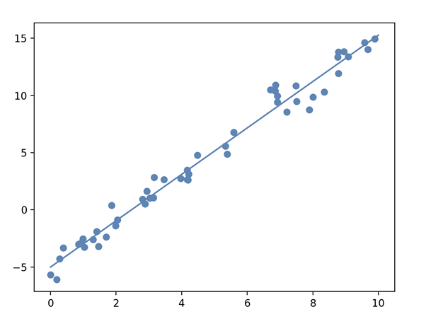
In this example, a linear regression model is created with random data, and an estimated regression line is displayed:

# Import the packages and classes needed for this example:
import numpy as np
import matplotlib.pyplot as plt
from sklearn.linear_model import LinearRegression
# Create random data with numpy:
rnstate = np.random.RandomState(1)
x = 10 * rnstate.rand(50)
y = 2 * x - 5 + rnstate.randn(50)
# Create a linear regression model based on the positioning of the data and Intercept, and predict a Best Fit:
model = LinearRegression(fit_intercept=True)
model.fit(x[:, np.newaxis], y)
xfit = np.linspace(0, 10, 1000)
yfit = model.predict(xfit[:, np.newaxis])
# Plot the estimated linear regression line with matplotlib:
plt.scatter(x, y)
plt.plot(xfit, yfit);
plt.show()

Figure 1. Estimated Linear Regression Line

Decision Tree Example

# Import the library required for this example
# Create the decision tree regression model:
from sklearn import tree
dtree = tree.DecisionTreeRegressor(min_samples_split=20)
dtree.fit(X_train, y_train)
print_accuracy(dtree.predict)


# Use Shap explainer to interpret values in the test set:
ex = shap.TreeExplainer(dtree)
shap_values = ex.shap_values(X_test)
# Plot Shap values:
shap.summary_plot(shap_values, X_test)

# Plot BMI (Body Mass Index) values: 
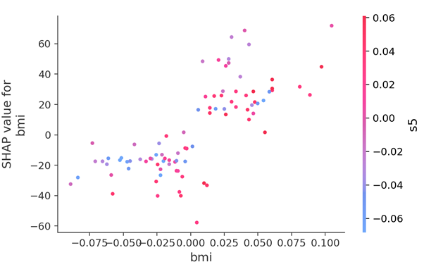
shap.dependence_plot("bmi", shap_values, X_test)

Figure 2.  BMI values distribution in a Shap Decision Tree

Random Forest Example

# Import the library required for this example
# Create a Random Forest regression model
# that implements a Fast TreeExplainer:
from sklearn.ensemble import RandomForestRegressor
rforest = RandomForestRegressor(n_estimators=1000, max_depth=None, min_samples_split=2, random_state=0)
rforest.fit(X_train, y_train)
print_accuracy(rforest.predict)


# Use Shap explainer to interpret values in the test set:
explainer = shap.TreeExplainer(rforest)
shap_values = explainer.shap_values(X_test)
# Plot Shap values:
shap.summary_plot(shap_values, X_test)

# Plot BMI values:
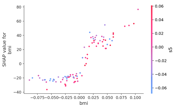
shap.dependence_plot("bmi", shap_values, X_test)

Figure 3.  BMI values distribution in a Shap Random Forest

Neural Network Example

# Import the library required in this example
# Create the Neural Network regression model:
from sklearn.neural_network import MLPRegressor
nn = MLPRegressor(solver='lbfgs', alpha=1e-1, hidden_layer_sizes=(5, 2), random_state=0)
nn.fit(X_train, y_train)
print_accuracy(nn.predict)

# Use Shap explainer to interpret values in the test set:
explainer = shap.KernelExplainer(nn.predict, X_train_summary)
shap_values = explainer.shap_values(X_test)
# Plot the Shap values:
shap.summary_plot(shap_values, X_test)

# Plot BMI values:
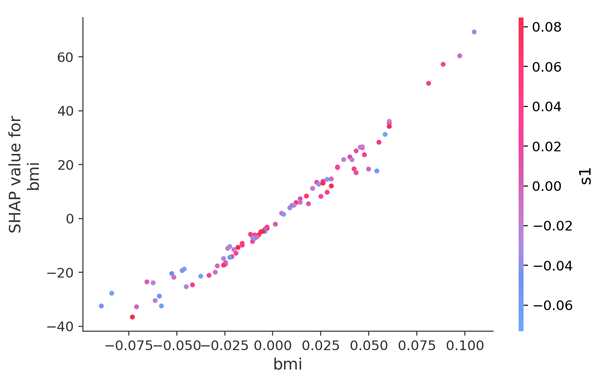
shap.dependence_plot("bmi", shap_values, X_test)

Figure 4.  BMI values distribution in a Shap Neural Network

Shap Regression Examples

In this set of examples, Shap values are applied to multiple regression models. Decision Tree, Random Forest, and Neural Network, are displayed in code blocks that share common libraries and classes:

# Import libraries required in the Shap examples, and load some data::
import sklearn
from sklearn.model_selection import train_test_split
import numpy as np
import shap
import time
X,y = shap.datasets.diabetes()
X_train,X_test,y_train,y_test = train_test_split(X, y, test_size=0.2, random_state=0)
# Summarize the training set with a subset of weighted kmeans, 
# each weighted by the number of points they represent:
X_train_summary = shap.kmeans(X_train, 10)
def print_accuracy(f):
    print("Root mean squared test error = {0}".format(np.sqrt(np.mean((f(X_test) - y_test)**2))))
    time.sleep(0.5) # Allow print() to take place before other processes.
shap.initjs()

Bayesian Ridge Example

Requirement: 

Bayesian Ridge regression requires the Python Bayesian-Optimization package. Enter the following command in a command-line or terminal to install the package:

pip install bayesian-optimization  
or
python -m pip install bayesian-optimization 

In this example, the BayesianRidge estimator class is used to predict new values in a regression model that lacks sufficient data. A linear regression is formulated using a probable distribution of values in the absence of actual values. The output, response ‘y’, is derived from the probable distribution rather than from actual values. 

# Import libraries needed in this example:
from sklearn.linear_model import BayesianRidge
from sklearn.datasets import load_boston
from sklearn.model_selection import train_test_split
from sklearn.metrics import mean_squared_error
import matplotlib.pyplot as plt
from numpy import sqrt
# Load the Boston Housing dataset: 
boston = load_boston()
# Split the data into x test, y train sets:
x, y = boston.data, boston.target
xtrain, xtest, ytrain, ytest=train_test_split(x, y, test_size=0.15)
# Define the BayesianRidge model with default parameters: 
bay_ridge = BayesianRidge()
# Fit the model with trained Bayesian data:
bay_ridge.fit(xtrain, ytrain)
# Use r-squared metrics to measure how close 
# the data is to the predicted regression line.
# Independent variable x^2 = score:
score=bay_ridge.score(xtrain, ytrain)
print("BayesianRidge regression model - score (r-squared mean): %.2f" % score)
# Predict the test data and check for accuracy: 
ypredict = bay_ridge.predict(xtest)
mse = mean_squared_error(ytest, ypredict)
# print("Mean squared error level: %.2f" % mse)
print("BayesianRidge regression - mean error level: %.2f" % sqrt(mse))

# Plot a BayesianRidge regression fitted to probable
# Bayesian values in relation to actual values:
xaxis = range(len(ytest))
plt.scatter(xaxis, ytest, s=8, color="blue", label="Actual values")
plt.plot(xaxis, ypredict, lw=0.8, color="red", label="Predicted regression")
plt.legend()
plt.show() 

The following tutorials will provide you with step-by-step instructions on how to work with machine learning Python packages:

• What is Scikit-learn in Python
• How to install Scikit-learn
• How to classify data in Python
• How to display a plot in Python
• How to build a Numpy array
• How to turn a Numpy array into a list
• How to label data for machine learning in Python
• How to run linear regressions in Python Scikit-Learn
• How to classify data in Python using Scikit-Learn

Get a version of Python, pre-compiled with Scikit-learn and other popular ML Packages

ActiveState Python is the trusted Python distribution for Windows, Linux and Mac, pre-bundled with top Python packages for machine learning – free for development use.

Some Popular ML Packages You Get Pre-compiled – With ActiveState Python

Machine Learning:

• TensorFlow (deep learning with neural networks)*
• scikit-learn (machine learning algorithms)
• keras (high-level neural networks API)

Data Science:

• pandas (data analysis)
• NumPy (multidimensional arrays)
• SciPy (algorithms to use with numpy)
• HDF5 (store & manipulate data)
• matplotlib (data visualization)

Get ActiveState Python for Machine Learning for Windows, macOS or Linux here.

Why use ActiveState Python instead of open source Python?

While the open source distribution of Python may be satisfactory for an individual, it doesn’t always meet the support, security, or platform requirements of large organizations.

This is why organizations choose ActiveState Python for their data science, big data processing and statistical analysis needs.

Pre-bundled with the most important packages Data Scientists need, ActiveState Python is pre-compiled so you and your team don’t have to waste time configuring the open source distribution. You can focus on what’s important–spending more time building algorithms and predictive models against your big data sources, and less time on system configuration.

ActiveState Python is 100% compatible with the open source Python distribution and provides the security and commercial support that your organization requires.

With ActiveState Python you can explore and manipulate data, run statistical analysis, and deliver visualizations to share insights with your business users and executives sooner–no matter where your data lives.