How To Run Linear Regressions In Python Scikit-learn

Scikit-learn is a Python package that simplifies the implementation of a wide range of Machine Learning (ML) methods for predictive data analysis, including linear regression.

Linear regression can be thought of as finding the straight line that best fits a set of scattered data points: 

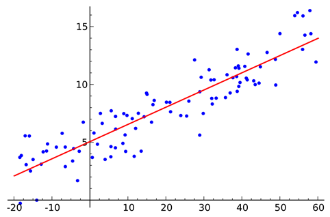
You can then project that line to predict new data points. Linear regression is a fundamental ML algorithm due to its comparatively simple and core properties.

Linear Regression Concepts

A basic understanding of statistical math is key to comprehending linear regression, as is a good grounding in ML concepts.

For more information on ML concepts and terminology, refer to: What is Scikit-Learn In Python?

The following are some key concepts you will come across when you work with scikit-learn’s linear regression method:

• Best Fit – the straight line in a plot that minimizes the deviation between related scattered data points.
• Coefficient – also known as a parameter, is the factor a variable is multiplied by. In linear regression, a coefficient represents changes in a Response Variable (see below).
• Coefficient of Determination – the correlation coefficient denoted as 𝑅². Used to describe the precision or degree of fit in a regression. 
• Correlation – the relationship between two variables in terms of quantifiable strength and degree, often referred to as the ‘degree of correlation’.  Values range between -1.0 and 1.0. 
• Dependent Feature – a variable denoted as y in the slope equation y=ax+b. Also known as an Output, or a Response. 
• Estimated Regression Line – the straight line that best fits a set of scattered data points.
• Independent Feature – a variable denoted as x in the slope equation y=ax+b. Also known as an Input, or a predictor. 
• Intercept – the location where the Slope intercepts the Y-axis denoted b in the slope equation y=ax+b. 
• Least Squares – a method of estimating a Best Fit to data, by minimizing the sum of the squares of the differences between observed and estimated values.
• Mean – an average of a set of numbers, but in linear regression, Mean is modeled by a linear function.
• Ordinary Least Squares Regression (OLS) – more commonly known as Linear Regression. 
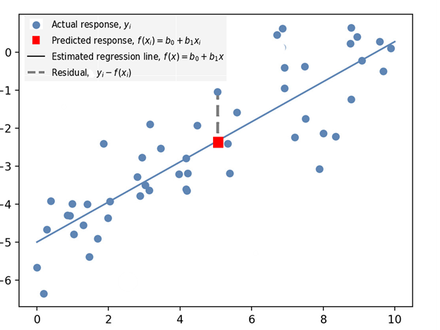
• Residual – vertical distance between a data point and the line of regression (see Residual in Figure 1 below).
• Regression – estimate of predictive change in a variable in relation to changes in other variables (see Predicted Response in Figure 1 below).
• Regression Model – the ideal formula for approximating a regression.
• Response Variables – includes both the Predicted Response (the value predicted by the regression) and the Actual Response, which is the actual value of the data point (see Figure 1 below).
• Slope – the steepness of a line of regression. Slope and Intercept can be used to define the linear relationship between two variables: y=ax+b.
• Simple Linear Regression – a linear regression that has a single independent variable.

Figure 1. Illustration of some of the concepts and terminology defined in the above section, and used in linear regression:

Linear Regression Class Definition

A scikit-learn linear regression script begins by importing the LinearRegression class:

from sklearn.linear_model import LinearRegression
sklearn.linear_model.LinearRegression()

Although the class is not visible in the script, it contains default parameters that do the heavy lifting for simple least squares linear regression:

sklearn.linear_model.LinearRegression(fit_intercept=True, normalize=False, copy_X=True)

Parameters: 

• fit_interceptbool, default=True

Calculate the intercept for the model. If set to False, no intercept will be used in the calculation.

• normalizebool, default=False

Converts an input value to a boolean. 

• copy_Xbool, default=True

Copies the X value. If True, X will be copied; else it may be overwritten.

How to Create a Linear Regression Model

In this example, a linear regression model is created based on data in a numpy array. The coefficients are formulated and then printed in the console:

# Import the packages and classes needed in this example:
import numpy as np
from sklearn.linear_model import LinearRegression
# Create a numpy array of data:
x = np.array([6, 16, 26, 36, 46, 56]).reshape((-1, 1))
y = np.array([4, 23, 10, 12, 22, 35])
# Create an instance of a linear regression model and fit it to the data with the fit() function:
model = LinearRegression().fit(x, y) 
# The following section will get results by interpreting the created instance: 
# Obtain the coefficient of determination by calling the model with the score() function, then print the coefficient:
r_sq = model.score(x, y)
print('coefficient of determination:', r_sq)
# Print the Intercept:
print('intercept:', model.intercept_)
# Print the Slope:
print('slope:', model.coef_) 
# Predict a Response and print it:
y_pred = model.predict(x)
print('Predicted response:', y_pred, sep='\n')

Watch how to create a Linear Regression and then print the Coefficients

How to Create a Linear Regression and Display it

In this example, random data is displayed in a plot. A linear regression model is then created against the data, and an estimated regression line is finally displayed.

# Import the packages and classes needed for this example:
import numpy as np
import matplotlib.pyplot as plt
from sklearn.linear_model import LinearRegression
# Create random data with numpy, and plot it with matplotlib:
rnstate = np.random.RandomState(1)
x = 10 * rnstate.rand(50)
y = 2 * x - 5 + rnstate.randn(50)
plt.scatter(x, y);
plt.show()
# Create a linear regression model based the positioning of the data and Intercept, and predict a Best Fit:
model = LinearRegression(fit_intercept=True)
model.fit(x[:, np.newaxis], y)
xfit = np.linspace(0, 10, 1000)
yfit = model.predict(xfit[:, np.newaxis])
# Plot the estimated linear regression line with matplotlib:
plt.scatter(x, y)
plt.plot(xfit, yfit);
plt.show()

Watch how to create a Linear Regression and display it in a Plot

Regression vs Classification 

The main difference between regression and classification is that the output variable in regression is continuous, while the output for classification is discrete. Regression predicts quantity; classification predicts labels. 

For information about classification, refer to:  How to Classify Data in Python

The following tutorials will provide you with step-by-step instructions on how to work with machine learning Python packages:

• What is Scikit-learn in Python
• How to install Scikit-learn
• How to classify data in Python
• How to label data for machine learning in Python
• How to build a Numpy array
• How to turn a Numpy array into a list

Get a version of Python, pre-compiled with Scikit-learn, NumPy, Pandas and other popular ML Packages

ActivePython is the trusted Python distribution for Windows, Linux and Mac, pre-bundled with top Python packages for machine learning – free for development use.

Some Popular ML Packages You Get Pre-compiled – With ActivePython

Machine Learning:

• TensorFlow (deep learning with neural networks)*
• scikit-learn (machine learning algorithms)
• keras (high-level neural networks API)

Data Science:

• pandas (data analysis)
• NumPy (multidimensional arrays)
• SciPy (algorithms to use with numpy)
• HDF5 (store & manipulate data)
• matplotlib (data visualization)

Get ActiveState Python for Machine Learning for Windows, macOS or Linux here.

Why use ActiveState Python instead of open source Python?

While the open source distribution of Python may be satisfactory for an individual, it doesn’t always meet the support, security, or platform requirements of large organizations.

This is why organizations choose ActivePython for their data science, big data processing and statistical analysis needs.

Pre-bundled with the most important packages Data Scientists need, ActiveState Python is pre-compiled so you and your team don’t have to waste time configuring the open source distribution. You can focus on what’s important–spending more time building algorithms and predictive models against your big data sources, and less time on system configuration.

ActiveState Python is 100% compatible with the open source Python distribution, and provides the security and commercial support that your organization requires.

With ActiveState Python you can explore and manipulate data, run statistical analysis, and deliver visualizations to share insights with your business users and executives sooner–no matter where your data lives.